Available with 3D Analyst license.
Ensuring data coverage and sampling density are common QA/QC tasks in workflows that involve the processing of lidar data. Identifying potential issues early on makes the task of mitigating the adverse impact of data shortcomings easier. The LAS dataset, along with two geoprocessing tools—Point File Information and LAS Point Statistics As Raster—are useful in this regard.
LAS dataset
Data for individual lidar projects is typically split into collections of tiled LAS files. This is done for the sake of processing convenience and to keep file sizes within reasonable limits. Unfortunately, this can turn into a hassle for someone working on one of these projects. The LAS dataset helps by allowing you to reference a project's collection of LAS files and operate on them as a whole. Use the Create LAS Dataset geoprocessing tool to make a LAS dataset.
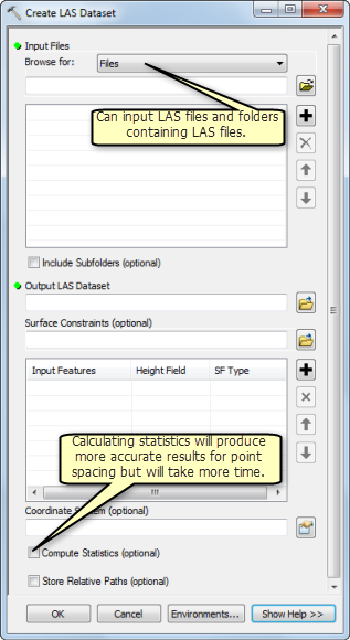
The Create LAS Dataset tool provides an option to compute statistics. If you do not specify this option, the LAS dataset is made quickly because only the header records of the referenced LAS files are read. Having the statistics computed requires a complete scan of the referenced LAS files. The time it takes to compute statistics corresponds to the number of points in the LAS files but yields much more information. For this reason, gathering statistics is highly recommended.
Once your LAS dataset is created, open the LAS Dataset Properties dialog box from the Catalog window. This dialog box reports information about the LAS dataset as a whole plus details about the specific LAS files that participate in the dataset. Go to the LAS Files tab of the dialog box.
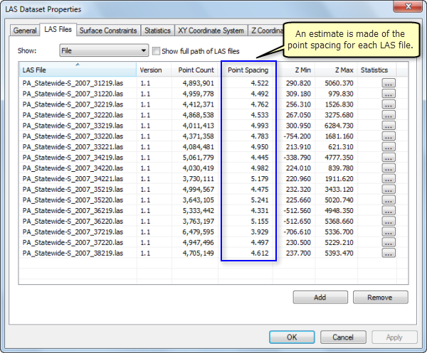
Look for the Point Spacing column in the middle of the LAS Files tab. This is the estimated point (in other words, return) spacing for each file. It is reported in the x,y units of the source data. The estimate is more accurate if you calculate statistics when creating the LAS dataset.
Point spacing is not the same as point density. Point spacing (PS) is defined as linear units per point, and point density (PD) is defined as points per square unit area. To convert point spacing to point density use the following equation: PD = 1/(PS)^2. A higher point density means lower values for point spacing.
Point File Information
The Point File Information tool reports basic statistics and extent information about point data files in LAS and ASCII formats and is a useful aid in the QA/QC process. Its output enables you to examine the point density, Z range, total point count, and georeferencing information for the input files, along with classification information for LAS files. When given a folder, the tool reads all files inside it that have the suffix you specify.
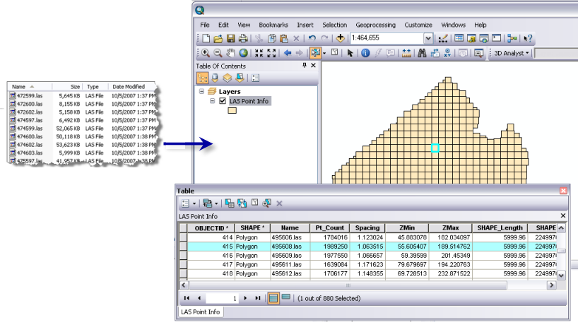
The point spacing reported by Point File Information is an approximation based on the area of the file's spatial extent divided by the total number of points in the file. It's most reliable when the data is evenly distributed throughout the file, but can otherwise offer misleading results with irregularly distributed data. In this situation, the reported point spacing is more meaningful as a summary when looking at trends for collections of files. However, the tool does offer an option to utilize an improved point spacing estimate for LAS files that mitigates the overestimation caused by irregular data distribution.
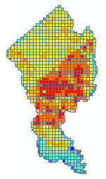
Symbolizing the point spacing field in the output feature using a graduated color ramp can provide a useful overview of trends in the data collection. In the image below, the LAS extent polygons are symbolized in this manner, and the polygons symbolized in red have a higher point density.
You can also review the classification of lidar points, which is typically performed by the lidar data provider. The classification used to distinguish between ground and nonground returns and is maintained using codes in the LAS files. The Summarize by Class Code option creates a unique feature for each class code in a LAS file. This provides a means for examining the class codes in each LAS file and the corresponding point information associated with each code. Checking the z-range specifically for a given class of points provides a more accurate representation of the data than if additional classes, like class 7, which represents noise points, were included in the analysis.
Assuming the Point File Information review process indicates the data is acceptable, the next step is to use the LAS Point Statistics As Raster geoprocessing tool to get a more in-depth view of the point distribution.
LAS Point Statistics As Raster
The LAS Point Statistics As Raster geoprocessing tool allows you to see the spatial distribution of different lidar point metrics. It does this by characterizing the points that fall into each cell of an output raster. You can choose to characterize the points in several ways:
- Pulse count
- Return count
- Predominant return count
- Maximum returns
- Predominant class
- Intensity range
- Z-range
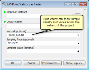
For the sake of assessing point coverage and density, pulse count is a good option. It assigns the number of last returns falling in a cell as the cell value. First, input a LAS dataset and pick PULSE_COUNT as the method. For sampling, choose CELLSIZE. You might think the average point spacing is a good cell size for the output raster, but this typically results in too many empty, or NoData, cells because lidar points are not evenly spaced. Also, the output raster could end up being unnecessarily large. Instead, it's better to go with a cell size that is several times larger than the average point spacing but small enough to identify gaps or voids that warrant further investigation. A reasonable size is four times the point spacing. For example, if your data is sampled at 1 meter and you set the cell size to 4, you can expect, on average, to get 16 pulses in a cell.
You can also evaluate the density for different types of points. While most of the time you'll probably just check the density for all returns, it can be useful to look at those that fall in a certain class. For example, looking at the pulse count for ground points can tell you how good your ground penetration is in vegetated areas. You can control what points are used by setting filtering criteria on the Filter tab of the LAS dataset layer. Point filter properties set on the layer are honored by the tool. If you use a dataset rather than a layer, there is no filtering.
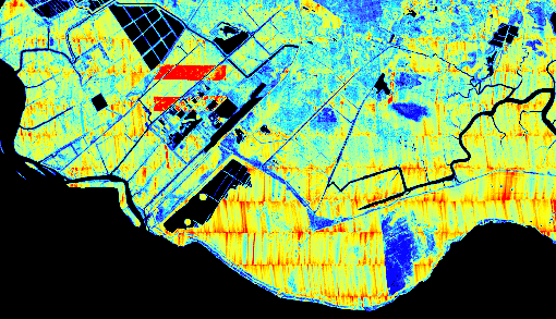
Once your raster has been created, look at it in ArcMap. Use a color ramp renderer to display it so it is easy to distinguish between cells with high counts and those with low. You can also set the NoData color to something that stands out. Look for variance in density and data voids. Have your vendor explain anything that doesn't look right.
In the image below, the black represents areas where NoData exists, while red represents areas where the lidar sample density is higher.
