Available with 3D Analyst license.
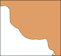
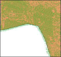
It is common for lidar or photogrammetric data for a survey to be delivered without a detailed data area boundary. Often, the x and y extents of the survey area are defined by a tile system that covers an area of interest, and the data fills these tiles. The image below depicts lidar data tiles for a project. The extent of these tiles is a gross approximation of the actual study area boundary.
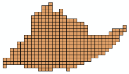
As is often the case, the actual lidar data does not fully cover the extent of tiles that are on the perimeter of the project area. The data is only guaranteed to cover some minimal extent, and there is no explicit or absolute boundary other than what can be inferred, as shown in the image below. This graphic is centered on one such tile.
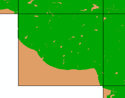
Either way, the area of coverage is usually not a cleanly filled rectangle.
The problem
If a surface is made without declaring the data area up front (in other words, by including a clip polygon when defining a terrain dataset or TIN), some of what are actually voids around the perimeter are treated as data areas. Analytic results in these areas are unreliable because height estimates are based on samples that can be far away.
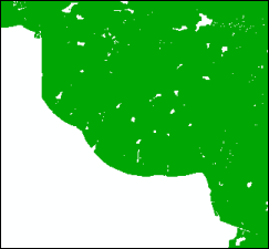
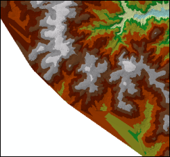
The graphic on the left below depicts a dense collection of lidar points shown in green. The gaps in the interior are water bodies (where lidar is typically omitted). The irregularly shaped data boundary is easy to see, but unless an explicit extent is provided in the form of a clip polygon, TIN, LAS dataset-, and terrain dataset-related tools will fill in voids, greatly oversimplifying the actual data extent.
You know areas outside the data collection extent should be excluded from the surface. The problem is coming up with the polygon that provides an accurate representation of this extent.
The solution
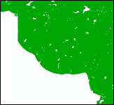
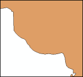
The solution is to synthesize a data boundary from the points that can be used to enforce a proper interpolation zone in the surface. Below, the left image depicts the lidar points. The middle image displays a polygon synthesized boundary from the points. The right image is a surface made from the lidar points and clip polygon.
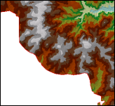
The point spacing is the primary variable to use when going after the data area. Surveys usually have explicit minimums on point spacing to provide control for interpolators. Areas that do not meet density requirements are exceptions. They usually fall in one of the following categories: water bodies, obscured areas, and holidays (send the latter back to the data provider for repair). The vast majority of the data will meet sample density specifications. Point spacing is usually reported in metadata. If you do not know the point spacing of the lidar data, see Assessing lidar coverage and sample density to learn how to determine it. Alternatively, display a zoomed-in view of the points using a LAS dataset and approximate the point spacing using the Measure tool in ArcMap. To learn more about point spacing, see Average point spacing.
Data area delineation from lidar points
Once you know the point spacing of the lidar data, follow these steps to delineate the data area:
- Rasterize the lidar points using the LAS Point Statistics As Raster geoprocessing tool.
Rasterization of the lidar points helps aggregate the area covered by the lidar points. It provides a good data structure to work with for subsequent steps. You just need to tell the geoprocessing tool what cell assignment type to use and the output cell size. Use PULSE_COUNT as the Method value for cell assignment. Specify a value for CELLSIZE that is several times larger than the average point spacing of the lidar data. Otherwise, you will get a lot of noise because the points are not evenly spaced. From the standpoint of processing efficiency and noise reduction, the larger cell size you use, the better, but there will be a trade-off with the tightness of fit in the result. A good place to start is four times the average point.
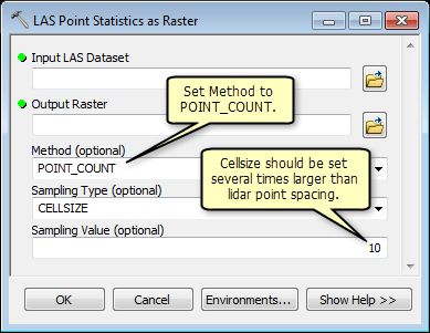
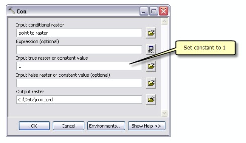
- Assign one value to all data cells using the Con geoprocessing tool.
Using the Con geoprocessing tool in this workflow simply turns any and all data cells of the raster into cells with one value. This value defines a raster zone that will be expanded in step 3. All that is needed is to take the output from the LAS Point Statistics As Raster tool and provide a constant value for a positive expression. All nonzero value cells will be considered positive and assigned the constant value. Since PULSE_COUNT was used as the cell assignment method during rasterization, any cell with a point in it must have a value greater than zero.
- Fill small NoData areas using the Expand geoprocessing tool.
Unless you used a very coarse cell size relative to your average point spacing, there is a likelihood of many NoData cells remaining. Most of these can be eliminated using the Expand geoprocessing tool. You want to remove them so the polygon produced during vectorization in a later step is not full of holes. That would be unnecessarily expensive.
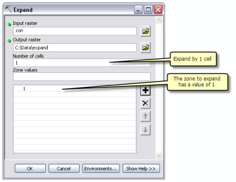
The Expand tool pushes the zone of interest outward. In this case, the zone is all the data cells coded with a value of 1. This effectively eliminates small gaps found in the interior.


The left image shows many individual cells and some small clusters of NoData cells (in white). The right image shows the results from using the Expand geoprocessing tool where the NoData cells (in white) are removed for the most part. It is okay if some isolated NoData areas remain in the output. The remaining NoData cells will be handled in the last step.
- Reduce the overall extent of data cells using the Shrink geoprocessing tool.
While Expand eliminates isolated NoData cells, it also extends the data area outward, so that needs to actually be brought in a little. Clip polygons need to be smaller than the actual point extent, so when terrain datasets or TINs try to estimate z-values along the polygon boundary, points can be found on both sides. This is needed to get good z-value estimates. To reduce the raster's data boundary, use the Shrink geoprocessing tool as shown below.
Reduce the extent somewhat so the polygon produced in step 5 is smaller than the actual data extent of the points. This enables the software to estimate better z-values along the polygon boundary.
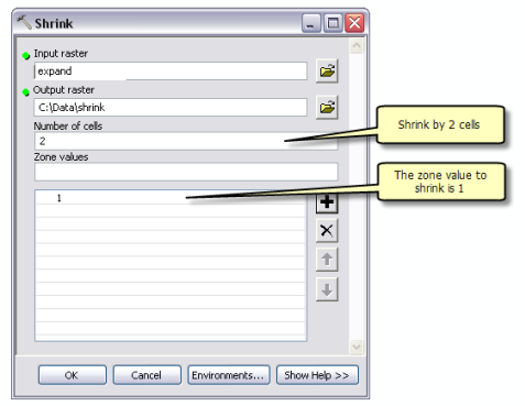
At this point, you have a relatively clean raster with the extent of its data cells slightly within the lidar point extent.
- Vectorize the raster with the Raster To Polygon geoprocessing tool.
The Raster To Polygon geoprocessing tool converts the raster to a polygon feature class. Make sure the Simplify polygons option is checked. If it is not, the output will be stairstepped rather than smooth and contain more vertices than necessary.
The Raster To Polygon tool outputs a polygon feature class. The result is representative of the data extent of the points used at the beginning of the process.
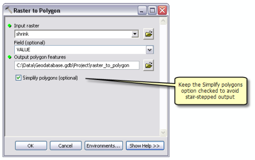
At this point, the process is almost complete. You need to review the output for correctness. Chances are there is one more step remaining, which is the removal of remaining holes inside your clip polygon.
- Remove any remaining small holes using the Eliminate Polygon Part geoprocessing tool.
The Eliminate Polygon Part geoprocessing tool eliminates any internal rings, leaving just the exterior boundaries.
A clip polygon now exists that can be added to a LAS dataset, terrain dataset, or TIN. It should conform to the data extent of the lidar points but fall slightly inside them. The left image below shows the resulting clip polygon. The right image is a zoomed-in view showing the extent of the polygon relative to the source points. Note how it lies slightly inside the source point boundary.
