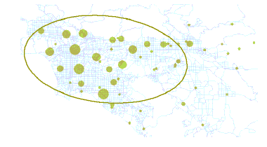
A common way of measuring the trend for a set of points or areas is to calculate the standard distance separately in the x- and y-directions. These two measures define the axes of an ellipse encompassing the distribution of features. The ellipse is referred to as the standard deviational ellipse, since the method calculates the standard deviation of the x-coordinates and y-coordinates from the mean center to define the axes of the ellipse. The ellipse allows you to see if the distribution of features is elongated and hence has a particular orientation.
While you can get a sense of the orientation by drawing the features on a map, calculating the standard deviational ellipse makes the trend clear. You can calculate the standard deviational ellipse using either the locations of the features or the locations influenced by an attribute value associated with the features. The latter is termed a weighted standard deviational ellipse.
Calculations
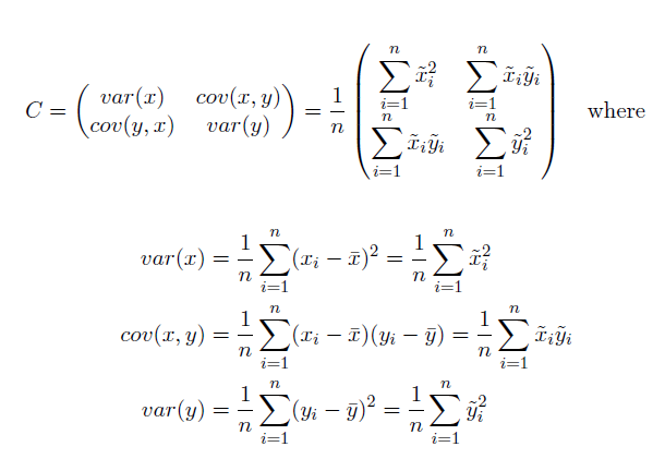
The Standard Deviational Ellipse is given as:

Where x and y are the coordinates for feature i, {x̄, ȳ} represent the Mean Center for the features and n is equal to the total number of features.
The sample covariate matrix is factored into a standard form which results in the matrix being represented by its eigenvalues and eigenvectors. The standard deviations for the x- and y-axis are then:

The variances are scaled by an adjustment factor in order to produce an ellipse containing the desired percentage of the data points. These adjustment factors are provided in the table below.
| 1 dimensional data | 2 dimensional data | |
|---|---|---|
1 standard deviation | 1.00 | 1.41 |
2 standard deviations | 2.00 | 2.83 |
3 standard deviations | 3.00 | 4.24 |
Visit the Additional resources if you would like to learn more about eigenvalues and eigenvectors.
Output and interpretation
Standard deviations help you understand the dispersion or spread of your data. When working with one dimensional data, the three sigma rule is the common rule-of-thumb conveying the percentage of data values that will fall within one, two and three standard deviations of the mean. In a normal distribution, this would mean 68%, 95% and 99.7% of the data values will fall within one, two and three standard deviations respectively. However, when working with higher dimensional spatial data (x and y), this breakdown of percentages is rarely observed. A more appropriate rule-of-thumb derived from the Rayleigh distribution suggests that a one standard deviational ellipse will cover approximately 63 percent of the features; two standard deviations will contain approximately 98 percent of the features; and three standard deviations will cover approximately 99.9 percent of the features in two dimensions (x and y).
For two dimensional data, the Directional Distribution (Standard Deviational Ellipse) tool creates a new feature class containing an elliptical polygon centered on the mean center for all features (or for all cases when a value is specified for Case Field). The attribute values for these output ellipse polygons include two standard distances (long and short axes); the orientation of the ellipse; and the case field, if specified. The orientation represents the rotation of the long axis measured clockwise from noon. You can also specify the number of standard deviations to represent (1, 2, or 3).

Potential applications
- Mapping the distributional trend for a set of crimes might identify a relationship to particular physical features (a string of bars or restaurants, a particular boulevard, and so on).
- Mapping groundwater well samples for a particular contaminant might indicate how the toxin is spreading and, consequently, may be useful in deploying mitigation strategies.
- Comparing the size, shape, and overlap of ellipses for various racial or ethnic groups may provide insights regarding racial or ethnic segregation.
- Plotting ellipses for a disease outbreak over time may be used to model its spread.
- Examining the distribution of elevations for storms of a certain category would be a useful factor to consider when investigating the relationship between atmospheric conditions and aircraft accidents.
Additional resources
Chew, Victor. "Confidence, prediction, and tolerance regions for the multivariate normal distribution." Journal of the American Statistical Association 61.315 (1966): 605-617.
Fisher, N. I., T. Lewis, and B. J. J. Embleton. Statistical Analysis of Spherical Data. 1st ed. Cambridge: Cambridge University Press, 1987. Cambridge Books Online. Web. 26 April 2016.
Levine, Ned. "CrimeStat III: a spatial statistics program for the analysis of crime incident locations (version 3.0)." Houston (TX): Ned Levine & Associates/Washington, DC: National Institute of Justice (2004).
Mitchell, Andy. The ESRI Guide to GIS Analysis, Volume 2. ESRI Press, 2005.
Wang, Bin, Wenzhong Shi, and Zelang Miao. (2015) Confidence Analysis of Standard Deviational Ellipse and Its Extension into Higher Dimensional Euclidean Space. PLoS ONE 10(3), e0118537.