Geostatistical Analyst のライセンスで利用可能。
There are three main components of Geostatistical Analyst:
- A set of exploratory spatial data analysis (ESDA) graphs
- The Geostatistical Wizard
- The Geostatistical Analyst toolbox, which houses geoprocessing tools specifically designed to extend the capabilities of the Geostatistical Wizard and allow further analysis of the surfaces it generates
The ESDA graphs and the Geostatistical Wizard are accessed through the Geostatistical Analyst toolbar, which must be added to the ArcMap display once the Geostatistical Analyst extension has been enabled (see Enabling the Geostatistical Analyst extension and Adding the Geostatistical Analyst toolbar to ArcMap).
Exploratory spatial data analysis graphs
Before using the interpolation techniques, you should explore your data using the exploratory spatial data analysis tools. These tools allow you to gain insights into your data and to select the most appropriate method and parameters for the interpolation model. For example, when using ordinary kriging to produce a quantile map, you should examine the distribution of the input data because this particular method assumes that the data is normally distributed. If your data is not normally distributed, you should include a data transformation as part of the interpolation model. A second example is that you might detect a spatial trend in your data using the ESDA tools and want to include a step to model it independently as part of the prediction process.
The ESDA tools are accessed through the Geostatistical Analyst toolbar (shown below) and are composed of the following:
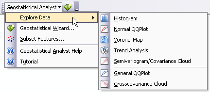
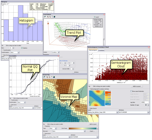
- Histogram—Examine the distribution and summary statistics of a dataset.
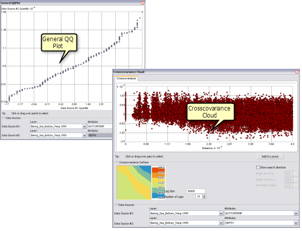
- Normal QQ Plot and General QQ Plot—Assess whether a dataset is normally distributed and explore whether two datasets have similar distributions, respectively.
- Voronoi Maps—Visually examine the spatial variability and stationarity of a dataset.
- Trend Analysis—Visualize and examine spatial trends in a dataset.
- Semivariogram/Covariance Cloud—Evaluate the spatial dependence (semivariogram and covariance) in a dataset.
- Crosscovariance Cloud—Assess the spatial dependence (covariance) between two datasets.
The ESDA graphs are shown below.
Tools for exploring a single dataset
The following graphic illustrates the ESDA tools used for analyzing one dataset at a time:
Tools for exploring relationships between datasets
The following graphic depicts the two tools that are designed to examine relationships between two datasets:
Geostatistical Wizard
The Geostatistical Wizard is accessed through the Geostatistical Analyst toolbar, as shown below:
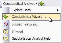
The Geostatistical Wizard is a dynamic set of pages that is designed to guide you through the process of constructing and evaluating the performance of an interpolation model. Choices made on one page determine which options will be available on the following pages and how you interact with the data to develop a suitable model. The wizard guides you from the point when you choose an interpolation method all the way to viewing summary measures of the model's expected performance. A simple version of this workflow (for inverse distance weighted interpolation) is represented graphically below:
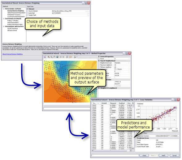
During construction of an interpolation model, the wizard allows changes in parameter values, suggests or provides optimized parameter values, and allows you to move forward or backward in the process to assess the cross-validation results to see whether the current model is satisfactory or some of the parameter values should be modified. This flexibility, in addition to dynamic data and surface previews, makes the wizard a powerful environment in which to build interpolation models.
The Geostatistical Wizard provides access to a number of interpolation techniques, which are divided into two main types: deterministic and geostatistical.
Deterministic methods
Deterministic techniques have parameters that control either (1) the extent of similarity (for example, inverse distance weighted) of the values or (2) the degree of smoothing (for example, radial basis functions) in the surface. These techniques are not based on a random spatial process model, and there is no explicit measurement or modeling of spatial autocorrelation in the data. Deterministic methods include the following:
- Global polynomial interpolation
- Local polynomial interpolation
- Inverse distance weighted
- Radial basis functions
- Interpolation with barriers (using impermeable or semipermeable barriers in the interpolation process)
Geostatistical methods
Geostatistical techniques assume that at least some of the spatial variation observed in natural phenomena can be modeled by random processes with spatial autocorrelation and require that the spatial autocorrelation be explicitly modeled. Geostatistical techniques can be used to describe and model spatial patterns (variography), predict values at unmeasured locations (kriging), and assess the uncertainty associated with a predicted value at the unmeasured locations (kriging).
The Geostatistical Wizard offers several types of kriging, which are suitable for different types of data and have different underlying assumptions:
These methods can be used to produce the following surfaces:
- Maps of kriging predicted values
- Maps of kriging standard errors associated with predicted values
- Maps of probability, indicating whether a predefined critical level was exceeded
- Maps of quantiles for a predetermined probability level
There are exceptions to this:
- Indicator and probability kriging produce the following:
- Maps of probability, indicating whether a predefined critical level was exceeded
- Maps of standard errors of indicators
- Areal interpolation produces the following:
- Maps of predicted values
- Maps of standard errors associated with predicted values
Geostatistical Analyst toolbox
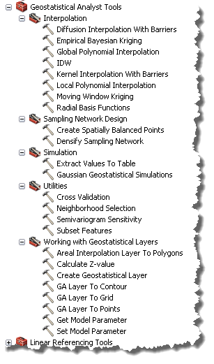
The Geostatistical Analyst toolbox includes tools for analyzing data, producing a variety of output surfaces, examining and transforming geostatistical layers to other formats, performing geostatistical simulation and sensitivity analysis, and aiding in designing sampling networks. The tools have been grouped into five toolsets:
- Interpolation—Contains geoprocessing tools that perform interpolation (as does the Geostatistical Wizard) that can be used as stand-alone tools or in ModelBuilder and Python
- Sampling Network Design—Has tools that aid in designing or modifying an existing sampling design/monitoring network
- Simulation—Extends kriging by performing geostatistical simulation and permits extraction of the simulated results for points or polygonal areas
- Utilities—General use tools to extract subsets of a dataset, perform cross-validation to assess model performance, examine sensitivity to variation in semivariogram parameters, and visually represent the neighborhoods used by the interpolation tools
- Working with Geostatistical Layers—Has tools that generate predictions for point locations, export geostatistical layers to raster and vector formats, retrieve and set interpolation model parameters (in an XML parameter file), and generate new geostatistical layers (based on an XML parameter file and datasets)
Subset Features
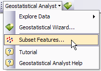
While cross-validation is provided for all methods available in the Geostatistical Wizard and can also be run for any geostatistical layer using the Cross Validation geoprocessing tool, a more rigorous way to assess the quality of an output surface is to compare predicted values with measurements that were not used to construct the interpolation model. As it is not always possible to go back to the study area to collect an independent validation dataset, one solution is to divide the original dataset into two parts. One part can be used to construct the model and produce a surface. The other part can be used to compare and validate the output surface. The Subset Features tool enables you to split a dataset into training and test datasets. The Subset Features tool is a geoprocessing tool (housed in the Geostatistical Analyst toolbox shown in the section above). For convenience, this tool is also available from the Geostatistical Analyst toolbar, as shown in the following figure:
For further information on this tool and how to use it, see How Subset Features works in Geostatistical Analyst and Using validation to assess models.
The process of building an interpolation model
Geostatistical Analyst includes many tools for analyzing data and producing a variety of output surfaces. While the reasons for your investigations might vary, you're encouraged to adopt the approach described in The geostatistical workflow when analyzing and mapping spatial processes:
- Represent the data—Create layers and display them in ArcMap.
- Explore the data—Examine the statistical and spatial properties of your datasets.
- Choose an appropriate interpolation method—The choice should be driven by the objectives of the study, your understanding of the phenomenon, and what you require the model to provide (as output).
- Fit the model—To create a surface. The Geostatistical Wizard is used in the definition and refinement of an appropriate model.
- Perform diagnostics—Check that the results are reasonable (expected), and evaluate the output surface using cross-validation and validation. This helps you understand how well the model predicts the values at unsampled locations.
Both the Geostatistical Wizard and Geostatistical Analyst toolbox offer many interpolation methods. You should always have a clear understanding of the objectives of your study and how the predicted values (and other associated information) will help you make more informed decisions when choosing a method. To provide some guidance, see Classification trees for a set of classification trees of the diverse methods.
(Data shown in the figures was provided courtesy of the Alaska Fisheries Science Center.)