Almost all GIS data is stored or represented as a simple database table. For example, feature classes are tables with a shape attribute (an attribute in a table is also termed a field or column), rasters can be viewed as tables of attributes, and most GIS databases have stand-alone tables containing attributes that can be related to other tables by a common attribute. When constructing a database or performing analysis, much of your time will be spent managing tables: adding and calculating new attributes, copying tables or their rows from one location to another, converting tables containing text strings of coordinate values into features, relating one table to another, or calculating summary statistics.
Some analyses require that GIS data be extracted as tables for another application, or tabular data from another application may become an input to the GIS. Often several geoprocessing steps modify and combine sets of data, resulting in a feature class with many attributes derived from other data, which can be selected or summarized to produce tabular results.
Creating GIS data from tables
Joining tables
One common technique is to join a table of data, such as demographic or medical statistics, to a set of geographic features for visualization. This requires that the table and the geographic features share a key field, such as a name or an ID code.
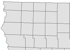
Below is an example of how GIS features can be given additional attributes by joining data from another table. This feature class of Iowa counties has name and FIPS code attributes that could be used as key fields for a table join.
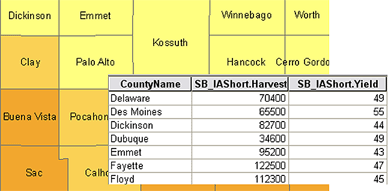
This stand-alone table contains information on the soybean harvest for each Iowa county. It has name and FIPS code attributes as well, so either could be used to join it to the county features.

After the harvest data is joined to the county features, you can use the fields from the harvest table to symbolize, label, or select the county features.
When you join data from different sources, it is important that the data types and values of the key fields match exactly. If one field is of numeric type and the other is text, it will not be possible to join using those fields. To work around this, you can create a new field in one of the tables that matches the data type in the other table, then calculate the values from the nonmatching field into the new, matching field. Also, if a key value is misspelled, has variant spellings, or contains a typographic error or extra characters (for example, a trailing space character), the records with unmatched keys will not be joined.
Making features from tables
Another common technique is to create spatial information from tabular data.
XY events
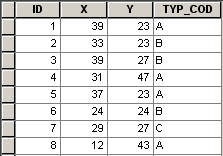
Perhaps the simplest method of doing this is by using the XY Event Layer tool to make a layer from a table that contains an x- and a y-coordinate field. Below is an example of how a simple table of coordinates and other data can be converted to point events.
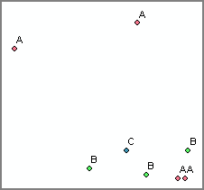
The point events created from the table behave just like a feature class and can be symbolized and labeled using attributes in the table.
Geocoding
You can also create points by matching values in a table against a reference feature class. One way of doing this is geocoding, where the table contains address information and the reference feature class contains street and area information.
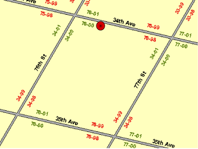
Below is an example of a point created from an address by geocoding the address against reference street data.
Linear referencing
Another way to do this is to match locations according to distance along a line, called linear referencing. This method can be used to create point events at a given distance along a line or line events that follow the line from a given location to another location.
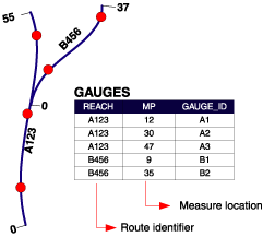
Below is an example of a set of point events generated by matching a table of distance measurements and route identifiers against a line feature class containing route features with measures.
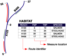
Below is an example of a set of line events generated by matching a table of from- and to-measurements and route identifiers against a line feature class containing route features with measures.
Analysis of tabular data
Analyzing tabular data often involves finding how many of something belong to a given category or looking at the distribution of values for a set of things. Often the particular things that you are interested in are surrounded by many others that are slightly (or very) different. Finding features based on those differences often involves combining data from different sources by joining tables or by spatial joins and overlays, then selecting and calculating values in fields.
Finding how many
Sometimes the features in your GIS have attributes that you want to analyze, by finding the sum of some field for selected features or the frequency of a particular feature type. The Summary Statistics and Frequency tools in the Statistics toolbox allow you to calculate these statistics on a field or several fields and to summarize the results according to values in yet another field. This can be useful for reporting as well as analysis.
Calculating frequency with the Frequency tool is a good way to learn how many of something fall into a given category. For example, you might run the tool on a set of parcels to see how many belong to each of several land-use categories. Looking at the frequency distribution of your categorical data is an important first step in many analyses.
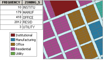
This frequency table tells you that there are almost five times as many residential parcels than office parcels and that a small minority of the parcels belong to the utility or institutional categories.
You can also get frequency information for a field in a table in ArcMap by right-clicking the header of the field in the table window and clicking Statistics.
Looking at the distribution of values
The Summary Statistics tool lets you quantify how much of something belongs to a set of features. For example, instead of just using Frequency to find out how many parcels there are of each type, you might use the Summary Statistics tool on the parcels to calculate the total (sum) area of parcels of each category or to find out how large, on average (mean), the parcels of each type are.
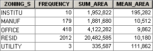
This summary statistics table tells you that although there are more manufacturing parcels than institutional parcels, each category covers a similar area of the city. It suggests that institutional and utility parcels tend to be larger than office, residential, or manufacturing parcels.
You can also use the Summary Statistics tool to examine the distribution of values for a set of features. For example, you could compare the minimum and maximum elevation values for several plant species in a study area, the range of prices for houses of a given type in an area, or the average amount that houses of that type differ from the average price (the standard deviation).
You can also summarize tables in ArcMap by right-clicking the column header of the field in the table window and clicking Summarize.
For more information on the use of statistics in GIS, see the Statistical analysis topic.
Counting records
Sometimes it is important to know how many records are in a table or a selection. You might use this information in a model or script that automates an analysis or reporting process. The Get Count tool returns the number of features or rows in a feature class, table, or layer. The tool respects selections, table views, and layers based on queries. You could use the Get Count tool in a looping script that buffers a location with a progressively greater distance and selects the features within the buffer until a given number of features have been selected.
Management of tabular data
Calculating values
The Calculate Field tool is used to mathematically combine or manipulate values in one or more fields. These calculations can be as simple as calculating a given field to 23 for all features or to true for all selected features or combining values in multiple fields. For example, you might divide a population field by an area field to get population density values or concatenate the text from house number, street name, and street type fields into a single address field. Many times, you want to add a new field using the Add Field tool to contain the results of your calculation.
Joining tables
The Add Join tool is often used to combine tabular data derived during one step of analysis with other data. If tables share a key value (a feature ID or name, for example), they can be joined. The data in both tables will then be available for simultaneous analysis. This tool only works on feature layers or table views in the ArcMap table of contents or created by the Make Feature Layer and Make Table View tools. The join is temporary and only lasts as long as the session. You can save the joined results to a new feature class or table by using the Copy Features or Copy Rows tools or by exporting the data in ArcMap.
Attribute indexes
Indexing a field can make the process of selecting rows with that attribute more efficient. You can use the Add Attribute Index tool to index a field.
Subtypes and attribute domains
When your table is stored in a geodatabase, you can create subtypes for your features and attributes. Subtypes provide a method of dividing your feature classes or tables into logical groupings based on an attribute value and allow you to work with a subset of features in a feature class or rows in a table. Subtypes make it possible to assign consistent attributes and behavior to those subsets.
Learn more about tools that create and manage subtypes
Domains offer a way to define a range of values that can be used for multiple attribute fields. Using domains helps ensure data integrity by limiting the choice of values for a particular field.
Table views
A table is a physical table on disk or in a database. A table view is a temporary table held in your computer's memory that you can use just like a physical table. Typically, you create a table view with a query, such as a SQL SELECT statement, so that only a subset of records of the physical table are in the table view.
The Make Table View tool creates a table view from one input table, while the Make Query Table tool creates a table view from many input tables that can be joined.
If you want to save a table view to a physical table, use the Copy Rows tool.
Pivoting a table
The Pivot Table tool allows you to reduce the redundancy in a large table. This is useful for converting certain CAD data structures into GIS features or for converting a long comma-delimited list of measurement stations and values to a table. Unique values in one field (the Pivot field) become column headings in the output table.
Raster tables
It's not uncommon for the pixel values of rasters to contain discrete integer values that classify its data, such as vegetation type. For example, a pixel value of 1 equals forestland while a pixel value of 2 represents wetlands. For such rasters, it's desirable to have a raster attribute table that describes each unique pixel value and to perform many of the table operations described above. The Build Raster Attribute Table tool creates or updates raster attribute tables.
Table tools
There are dozens of tools that manage and manipulate tables and their attributes. Most of these tools are found in the Data Management toolbox.
| Toolbox | Description |
|---|---|
Contains the Frequency and Summary Statistics tools | |
Converts data to ArcGIS formats | |
Allows tables of addresses to be converted to point features | |
Allows tables containing [route, measure] coordinates to be converted to point features |