Exercise 3: Finding a site for a new school

Available with Spatial Analyst license.

Complexity:

Beginner

Data Requirement:

ArcGIS Tutorial Data for Desktop

In this exercise, you'll build a suitability model with ArcGIS Spatial Analyst tools that finds suitable locations for a new school. The steps to produce such a suitability model are outlined below.

Your input datasets in this exercise are landuse, elevation, rec_sites, and schools. You will derive slope, distance to recreation sites, and distance to existing schools. Then you'll reclassify these derived datasets to a common scale from 1 to 10. You'll weight them and the landuse dataset according to a percentage of influence, and combine them to produce a map displaying suitable locations for the new school. You'll then select the optimal site for the new school from the alternatives.

This exercise will take approximately 45 minutes to complete. Start this exercise with your Site Analysis map document, created in exercise 1, open.

Creating a new toolbox

You'll first create a new toolbox to hold the models you'll create in this exercise and the next exercise.

1. Create a new toolbox in your Spatial Analyst folder. Name the toolbox Site Analysis Tools.

   Tip:

   For more information on creating a toolbox, see Creating a custom toolbox.

Creating a new model

You'll create a model to perform Spatial Analyst tasks. A model is built by stringing tools together in ModelBuilder. Once your model is created, you can easily experiment with parameter values, use different input data, run the model over and over again, and share it with others. To find out more about ModelBuilder, see What is ModelBuilder.

In this exercise, you'll create a model to find a suitable location for a new school.

1. Right-click the Site Analysis Tools toolbox and click New > Model.

   

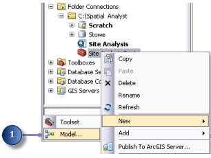
   An empty ModelBuilder session opens.

Renaming the model

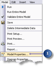
1. On the model's main menu, click Model > Model Properties.

   

2. Click the General tab.
3. Type FindSchool in the Name text box and Find location for school in the Label text box.

   The name is used in scripting and at the Python window. The label is the display name for the model.

4. Check the Store relative path names (instead of absolute paths) check box.

   

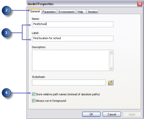
   Checking this box sets all source paths referenced by the tool as relative to the location of the toolbox; therefore, if the model is moved to a different directory, it will still be able to be executed successfully.

Specifying environment settings

Before you perform analysis on your data, you should set any relevant environment settings. For more information on how to set environments and the hierarchy between analysis environments, see The analysis environment of the ArcGIS Spatial Analyst.

Because your environment settings apply to each process of this model only, you'll set environment settings for the model.

1. Click the Environments tab.
2. Expand Processing Extent and check Extent.
3. Expand Raster Analysis and check Cell Size.

   Tip:

   The Current Workspace and the Scratch Workspace are already set, as these environment settings are inherited from the map document.

4. Click Values.

   

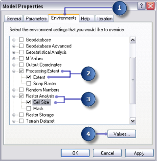
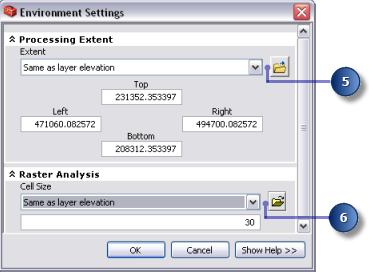
5. Expand Processing Extent. Set the Extent by clicking the drop-down arrow and choosing Same as Layer elevation.
6. Expand Raster Analysis. Set the Cell Size by clicking the drop-down arrow and choosing Same as Layer elevation.

   The cell size of your elevation layer will be applied to all subsequent raster outputs. Your elevation dataset has the largest cell size (30 meters).

   Caution:

   Setting a smaller cell size than your largest input will not mean you have more detailed information in subsequent raster results; you will just have more cells of the same value, which may affect your display and calculation speeds. Although the software does not prevent it, it is considered incorrect to set a cell size smaller than your largest input cell size.

7. Click OK in the Environment Settings window.

   

8. Click OK in the Model Properties window.
9. On the toolbar, click the Save button .

   Tip:

   The model's properties are updated. If at any point you want to close the model and continue later, right-click the model in the ArcToolbox window and click Edit to continue with the tutorial.

Deriving datasets

You are ready to process your project data to locate suitable areas for the new school. You'll derive the following from your project data:

• Slope from the elevation dataset
• Distance from recreation sites from the rec_sites dataset
• Distance from existing schools from the schools dataset

This first section of your model will look like the following: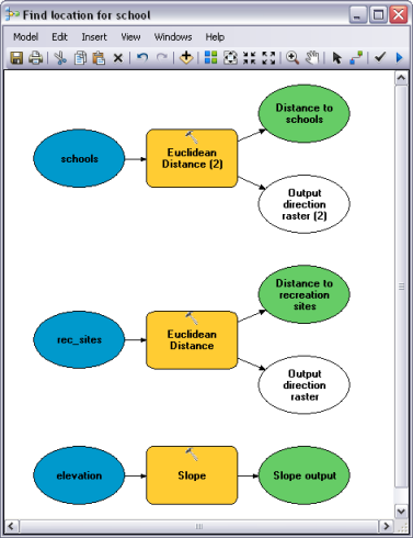

1. From your table of contents, drag the layers elevation, rec_sites, and schools onto your model.
2. Click and drag the Slope tool from the Spatial Analyst Surface toolset onto your model and place it in line with your elevation data.

   An element that references the Slope tool is created in the display window.

3. Locate the Euclidean Distance tool in the Spatial Analyst Tools toolbox Distance toolset. Click and drag the Euclidean Distance tool onto your model and place it in line with rec_sites.
4. Repeat the previous step, but this time place the Euclidean Distance tool in line with schools.

   Notice that each time the same tool is added to a model, the name of the tool element is appended with a number. The second time Euclidean Distance was added to your model, the label consisted of the tool name followed by (2). You can change these labels if you want, but it's unnecessary for this example.

   

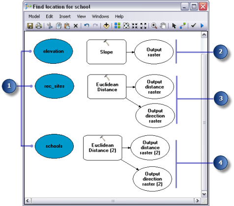
5. Click the Add Connection tool .
6. Use the Add Connection tool to connect the elevation dataset to the Slope tool. To do this, click elevation, then click the Slope tool, after which you'll see a pop-up menu. Choose Input raster.
7. Repeat the previous step, this time connecting rec_sites to the Euclidean Distance tool and choosing Input raster or feature source data on the pop-up menu. Do the same to connect schools to the Euclidean Distance (2) tool.

   Note:

   The process (consisting of the input data, tool, and default output data elements) is now filled with a solid color, meaning it's ready to run. The direction output element of Euclidean Distance is uncolored, since it's optional and by default is left undefined in the tool. If you were to run the model now, it would run using the default parameters for each tool.

8. On the model toolbar, click the Select tool , because you no longer need the Add Connection tool.
9. Click the Auto Layout button , then click the Full View button to apply the current diagram properties to the elements and place them within the display window.
10. On the toolbar, click the Save button .

    

Deriving slope from elevation

Since the area is mountainous, you need to find areas of relatively flat land on which to build, so you'll take into consideration the slope of the land.

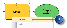
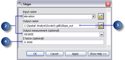
1. Right-click the Slope tool and click Open, or double-click the Slope tool.

   

2. Leave the Input raster and the Output measurement as the default values.
3. Accept the default location for the value of the Output raster parameter, but type slope_out for the name.

   A meaningful output name, slope_out, has been provided to help locate this data later in exercise 3.

4. For the Z factor, type 0.3048 to convert the z-values to the same unit of measure as the x,y units (from feet to meters).
5. Click OK.

   

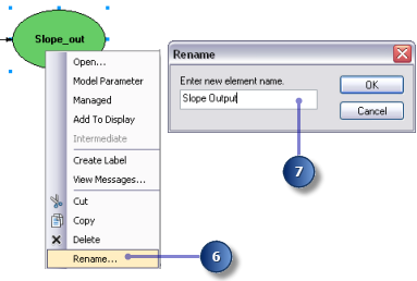
6. Right-click the output variable from the Slope tool and click Rename.
7. Type Slope Output then click OK.

   

   Caution:

   Renaming an element label does not alter the name of the output on disk. A layer will be added to the Table of Contents called Slope Output, which references data on disk called Slope_out.

Deriving distance from recreation sites

To find locations close to recreation sites, you must first calculate the Euclidean (straight-line) distance from recreation sites.

1. Hover over the Euclidean Distance tool connected to rec_sites. You can see all the default parameters set for this tool. There is no need to adjust any of these parameters.

   

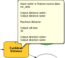
   You accepted the default for the Maximum distance, thus leaving this parameter empty. Therefore, the edge of the output raster is used as the maximum distance. The Output cell size is taken from the environment setting previously set to that of your elevation data. In this exercise, the Output direction raster is not required.

2. Rename the output variable from the Euclidean Distance tool Distance to recreation sites.

Deriving distance from schools

To find locations away from existing schools, you must first calculate the Euclidean (straight-line) distance from schools.

1. Hover over the Euclidean Distance (2) tool connected to schools. You can see all the default parameters set for this tool. There is no need to adjust any of these parameters.
2. Rename the output variable from the Euclidean Distance (2) tool Distance to schools.

Run model to derive datasets

1. Right-click each of the output variables (Slope output, Distance to recreation sites, and Distance to schools) then click Add To Display.

   

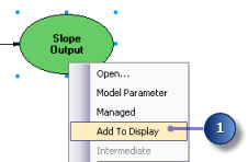
   With the Add To Display property on, the data referenced by the variable will be added to the display each time the model is run.

2. Click the Run button on the model toolbar to execute the three tools—Slope, Euclidean Distance, and Euclidean Distance (2)—in your model.

   Notice that as the tool runs, its progress is documented on the progress dialog box, and the tool that references the tool is highlighted in red. When the tools have finished running, the tool and its output become shaded, indicating that the output has been created on disk.

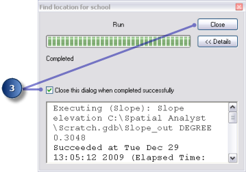
3. If the progress dialog box is present, check the Close this dialog when completed successfully check box, then click Close.

   

4. Examine the layers added to your ArcMap display.

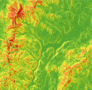
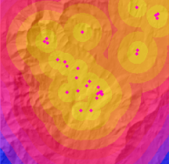
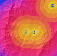
   For a better view, you can change the transparency of the target reviewing layer, and display the hillshade layer (created in Exercise 2) under it to have a vivid impression of the terrain, just like the result maps below. For example, to view the Distance to recreation sites layer, in the table of contents, click and drag the rec_sites layer over the Distance to recreation sites layer, and drag the hillshade layer under that. Uncheck unnecessary layers in the table of contents. Then change the transparency of the Distance to recreation sites layer from the default of 0 to 30. You'll see results like the Distance from recreation sites map showed below.

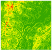
On the Slope Output layer, steep slopes are displayed in red and less steep slopes in green in the output layer. On the Distance to recreation sites layer, distances increase the farther you are from a recreation site. On the Distance to schools layer, distances increase the farther you are from a school.

Slope output map

Distance from recreation sites map

Distance from schools map

Reclassifying datasets

Deriving datasets, such as slope, is the first step when building a suitability model. Each cell in your study area now has a value for each input criteria (slope, land use, distance to recreation sites, and distance to schools). You need to combine the derived datasets so you can create your suitability map, which will identify the potential locations for the new school. However, it is not possible to combine them in their present form—for example, combining a cell value in which slope equals 15 degrees with a cell value for land use that equals 7 (forest)—and get a meaningful answer that you can compare to other locations. To combine the datasets, they first need to be set to a common measurement scale, such as 1 to 10. That common measurement scale is what determines how suitable a particular location—each cell—is for building a new school. Higher values indicate more suitable locations for the school.

Using the Weighted Overlay tool, you can weight the values of each dataset, and then combine them. However, the inputs for the Weighted Overlay tool must contain discrete, integer values. Land-use data is already categorized into discrete values; for example, forest equals a value of 7, so you can add this dataset directly into the Weighted Overlay tool and assign each cell a new value on the common measurement scale of 1 to 10 (you'll do this later in the tutorial). The values in the datasets you derived in previous steps are all floating-point, continuous datasets, categorized into ranges, and they must first be reclassified so that each range of values is assigned one discrete integer value. Potentially, the value given to each range can be any number, provided you note the range that the value corresponds to. This is because you can weight these values within the Weighted Overlay tool—the next step after reclassifying the derived datasets. However, it's easier to weight the cell values for derived datasets while reclassifying. In the Weighted Overlay tool, you can accept the default and leave the scale values the same as the input values.

You'll reclassify each derived dataset to a common measurement scale, giving each range a discrete integer value between 1 and 10. Higher values will be given to attributes within each dataset that are more suitable for locating the school.

This section of your model will look like the following: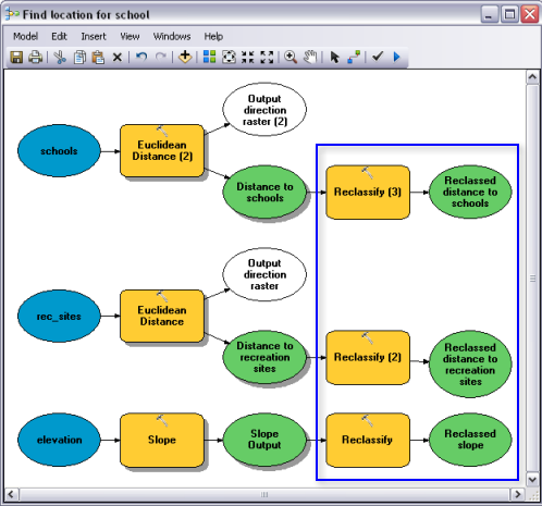

1. Locate the Reclassify tool in the Spatial Analyst Tools toolbox Reclass toolset. Click and drag the Reclassify tool onto ModelBuilder in line with Slope Output. Add another Reclassify tool in line with Distance to recreation sites and another in line with Distance to schools.
2. Click the Add Connection tool . Use the connect tool to connect the following:
   1. Slope Output to the Reclassify tool
   2. Distance to recreation sites to the Reclassify (2) tool
   3. Distance to schools to the Reclassify(3) tool
3. On the model toolbar, click the Select tool .
4. Click the Auto Layout button , then click the Full View button .

Reclassifying slope

It is preferable that the new school site be located on relatively flat ground. You'll reclassify the slope output, slicing the values into equal intervals. You'll assign a value of 10 to the most suitable range of slopes (those with the lowest angle of slope) and 1 to the least suitable range of slopes (those with the steepest angle of slope) and linearly rank the values in between.

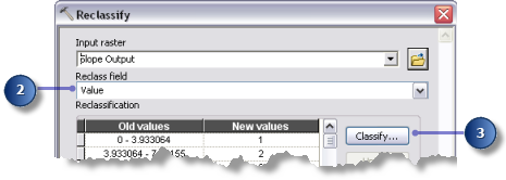
1. Open the Reclassify tool connected to the Slope Output variable.
2. Accept the default for the Reclass field parameter so the Value field will be used.
3. Click Classify.

   

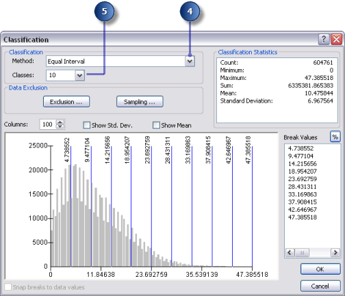
4. Click the Method drop-down arrow and click Equal Interval.
5. Click the Classes drop-down arrow and click 10.
6. Click OK.

   

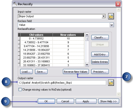
7. Click Reverse New Values.

   Reversing the values applies higher new values to the values representing less steep slope, since these areas are more suitable for building.

8. Accept the default for the Output raster parameter.
9. Click OK.

   

10. Rename the output variable from the Reclassify tool to Reclassed slope.

Reclassifying distance to recreation sites

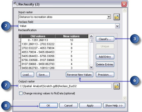
The school should be located as close as possible to a recreational facility. You'll reclassify the distance to recreation sites output, assigning the number 10 to ranges of values that represent areas closest to recreation sites (the most suitable locations), assigning the number 1 to ranges of values that represent areas far from recreation sites (the least suitable locations), and ranking the values linearly in between.

1. Open the Reclassify tool connected to the Distance to recreation sites variable.
2. Accept the default for the Reclass field parameter so the Value field will be used.
3. Click Classify.
4. Set the Method to Equal Interval and the number of Classes to 10.
5. Click OK.
6. Click Reverse New Values.

   Clicking Reverse New Values makes it so that distances close to recreational facilities receive a higher new value, since these areas are more desirable.

7. Accept the default path and name for the Output raster parameter.
8. Click OK.

   

9. Rename the output variable from the Reclassify (2) tool Reclassed distance to recreation sites.

   Tip:

   To resize the output variable element, Reclassed distance to recreation sites, click the element and move the mouse pointer over one of the blue handles surrounding the element, then click and drag to resize the element so all text can be seen.

Reclassifying distance to schools

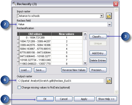
It's necessary to locate the new school away from existing schools to avoid encroaching on their catchment areas. You'll reclassify the Distance to schools layer, assigning a value of 10 to areas farthest from existing schools (the most suitable locations), assigning a value of 1 to areas near existing schools (the least suitable locations), and linearly ranking the values in between. By doing this, you'll determine which areas are near and which areas are far from existing schools.

1. Open the Reclassify (3) tool.
2. Accept the default for the Reclass field parameter so the Value field will be used.
3. Click Classify.
4. Set the Method to Equal Interval and the number of Classes to 10.
5. Click OK.

   You want to position the school away from existing schools, so you'll assign larger numbers to ranges of values that represent locations farther away, because these locations are most desirable. Since the default assigns high New values (more suitable locations) to higher ranges of Old values (locations farther away from existing schools), you do not need to change any values at this time.

6. Accept the default for the Output raster parameter.
7. Click OK.

   

8. Rename the output variable from the Reclassify (3) tool Reclassed distance to schools.

Executing the Reclassify operation

1. Right-click each of the variable outputs—Reclassed slope, Reclassed distance to recreation sites, and Reclassed distance to schools—and click Add To Display.
2. Click the Run button to execute the three Reclassify tools in your model.
3. On the toolbar, click the Save button .
4. Examine the layers added to your ArcMap display. To have a better view, you can, for example drag the rec_sites layer over the reclassified distance to recreation sites layer, so you can see the 10 distance rings starting from the origins of recreation sites. You can customize your map by changing points symbology, such as the map shown below. Do the same to the reclassified distance to schools layer.

   

   Reclassified slope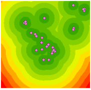

   

   Reclassified distance to recreation sites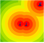

   

   Reclassified distance to schools

   

   Legend

   Locations with higher values (with low gradient slopes, close to recreation sites, and away from existing schools) are more suitable than locations with lower values (with steeper slopes, far from recreation, and close to existing schools ).

Weighting and combining datasets

You are now ready to combine the reclassified datasets and land use to find the most suitable locations. The values of the reclassified datasets representing slope, distance to recreation sites, and distance to schools have all been reclassified to a common measurement scale (more suitable cells have higher values). The landuse dataset is still in its original form because you can weight the cell values for this dataset as part of the weighted overlay process. Values representing areas of water and wetlands will be restricted. You'll also mark slope values that are less than 4 (the least suitable because they are too steep) as restricted so these values can be excluded. If all datasets were equally important, you could simply combine them, giving each equal influence; however, you've been informed that it's preferable to locate the new school close to recreational facilities and away from other schools. You'll weight all the inputs, assigning each a percentage of influence. The higher the percentage, the more influence a particular input will have in the suitability model.

You'll assign the inputs the following percentages of influence:

Reclassed distance to rec_sites: 50%
Reclassed distance to schools: 25%
Reclassed slope: 13%
landuse: 12%

This section of your model will look like the following: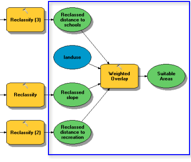

1. Click and drag the Weighted Overlay tool, located in the Spatial Analyst toolbox Overlay toolset, into ModelBuilder.

Setting up the Weighted Overlay operation

1. Open the Weighted Overlay tool.
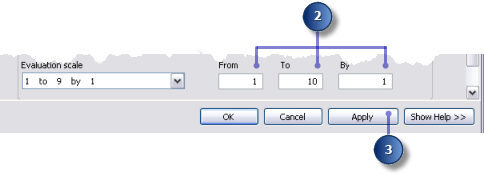
2. Type 1, 10, and 1 in the From, To, and By text boxes, respectively.

   The default evaluation scale is from 1 to 9 by 1. A scale of 1 to 10 was used when reclassifying datasets, so before adding input rasters to the Weighted Overlay tool, you want to set the evaluation scale from 1 to 10 by 1. This means you'll avoid having to update the scale values after adding your input datasets.

3. Click Apply.

   

4. Add the Reclassed slope to the Weighted Overlay tool.
   1. Click the Add raster row button .
   2. For the input raster, choose Reclassed slope from the drop-down list and leave the input field as Value.
   3. Click OK.

   

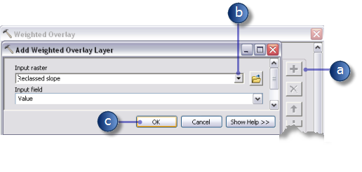
   The raster is added to the Weighted Overlay Table. The Field column displays the values of the Reclassed slope data. The Scale Value column mimics the Field column because the Evaluation scale was set to encompass the range of values in each input raster. You could modify the Scale Values for each class at this point, but for this input, the values were already weighted appropriately at the time of reclassifying.

5. Repeat the previous step for each of the reclassified datasets, including Reclassed distance to schools and Reclassed distance to recreation sites.
6. For the Reclassed slope input, in the Scale Value column, click the cell with a value of 1.
7. Click the drop-down arrow, scroll down, and click Restricted.

   

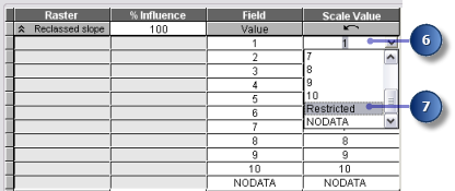
   You know you don't want to build on slopes greater than about 33 percent, even if all other conditions are ideal. You'll make values from 1 to 3 restricted, since these values represent slopes from 33.431043 to 47.758633 (the maximum slope).

   Dive-in:

   Setting a Scale Value to Restricted assigns a value to that cell in the output weighted overlay result that is the minimum value of the evaluation scale set minus 1 (zero in this exercise). If there are no inputs to the Weighted Overlay tool with cells of NoData, you could use NoData as the scale value to exclude certain values. However, if you have NoData cells in any of your inputs, it is safest to use Restricted. Potentially, a result from the Weighted Overlay tool could contain cells of NoData that have come from one or more of the inputs (NoData on any input equals NoData in the result) and restricted areas that you intentionally excluded. NoData and Restricted values should not be confused. Each serves a specific purpose. There may be areas of NoData for which you don't know the value but that are actually suitable areas. If you use NoData to exclude certain cell values and there is NoData in one or more inputs, you will not know whether a cell of NoData means the area is restricted from use or there was no input data available in that location.

8. Set Scale Values of 2 and 3 to Restricted.
9. Add the landuse layer, this time setting the Input field to LANDUSE. Click OK.

   You'll now weight the scale values of the landuse layer so they are comparable with the other inputs. A lower value indicates that a particular land-use type is less suitable for building. The scale values for Water and Wetlands will be set as Restricted, since they cannot be built on and should be excluded.

10. Change the default Scale Values for the landuse layer to the following values:
    • Brush/transitional—5
    • Barren land—10
    • Built up—3
    • Agriculture—9
    • Forest—4

11. Set the Scale Values representing Water and Wetlands to Restricted.
12. Collapse each raster in the Weighted overlay table.

    

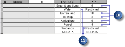
    You'll now assign a percentage of influence to each raster, based on how much importance (or weight) each should have in the final suitability map.

13. In the % Influence column, type the percentages for each of the input rasters as follows:
    • Reclassed slope to 13
    • Reclassed distance to schools to 25
    • Reclassed distance to recreation sites to 50
    • Reclassed landuse to 12

    

    Tip:

    Move the mouse pointer over the name of an input raster to view the entire name.

14. Accept the default for the Output raster parameter.
15. Click OK.

Executing the Weighted Overlay operation

1. Click the Auto Layout button , then click the Full View button .
2. Rename the output variable from the Weighted Overlay tool to Suitable Areas then click OK.
3. Right-click the Suitable Areas variable and click Add To Display.
4. Run the Weighted Overlay tool.
5. On the toolbar, click the Save button .

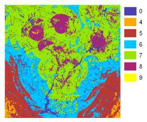
Examine the layer added to your ArcMap display. Locations with higher values indicate more suitable sites—areas that are on less steep slopes of suitable land-use types, closer to recreational facilities, and away from existing schools. Notice that the areas you marked as restricted have a value of zero.

Suitable Areas map

Selecting optimal sites

On your layer, each pixel has a value that indicates how suitable that location is for a new school. Pixels with the value of 9 are most suitable, and pixels with the value of 0 are not suitable. Therefore, the optimal site location for a new school has the value of 9. Another criteria for an optimal location is the size of the suitable area. A suitable location would include several pixels with value of 9 being connected.

This section of your model will look like the following:

Extract optimal sites using the Con tool

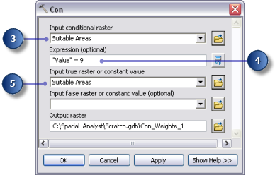
You'll use a conditional expression in the Con tool to extract only the optimal sites. It's been decided that those sites that are considered optimal must have a suitability value of 9 (the highest value in the suit_areas output). In the conditional expression, all areas with a value of 9 will retain their original value (9). Areas with a value of less than 9 will be changed to NoData.

1. Click and drag the Con tool, located in the Conditional toolset, into ModelBuilder.
2. Open the Con tool.
3. Click the Input Conditional Raster value drop-down arrow and click the Suitable Areas variable.
4. Type the condition Value = 9 for the value of the Expression parameter.
5. Click the Input true raster or constant value drop-down arrow and click the Suitable Areas variable.

   If the condition you enter is true, then the value of the cells of the Input true raster or constant value will be applied to the cells of the output raster.

6. Leave the value for the Input false raster or constant value parameter blank.

   Leaving the Input false raster or constant value parameter blank will apply the default. The default is that any value in the Input conditional raster that doesn't meet the condition you enter will be assigned NoData in the output raster.

7. Accept the default for the Output raster parameter.
8. Click OK.

   

9. Click the Auto Layout button , then click the Full View button .
10. Rename the output variable from the Con tool Optimal areas then click OK.
11. Right-click Optimal areas and click Add To Display.
12. Run the Con tool.

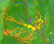
Examine the layer added to your ArcMap display. These are the optimal site locations for the new school. There are many single cells representing optimal locations. These 30-meter cells are too small for the school site. You'll clean up the result, removing these small areas, using the Majority Filter tool.

Refine the optimal areas using the Majority Filter tool

1. Click the Majority Filter tool, located in the Spatial Analyst Tools toolbox Generalization toolset, and add it to ModelBuilder.
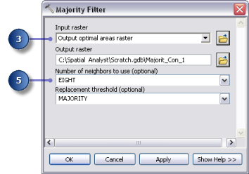
2. Open the Majority Filter tool.
3. Click the Input raster drop-down arrow and click the Optimal areas raster variable.
4. Accept the default Output raster parameter.
5. Click the Number of neighbors to use drop-down arrow and click EIGHT.

   This option specifies the number of neighboring cells to use in the kernel of the filter. The kernel of the filter will be the eight nearest neighbors (a 3-by-3 cell window) to the present cell.

6. Accept the default to use MAJORITY as the Replacement threshold.

   Using MAJORITY as the Replacement threshold means five out of eight connected cells must have the same value for the present cell to retain its value.

7. Click OK.

   

8. Rename the output variable from the Majority Filter tool Filtered optimal areas.
9. Right-click the Filtered optimal areas and click Add To Display.
10. Run the Majority Filter tool.
11. On the toolbar, click the Save button and close your model.

Examine the layer added to your ArcMap display. Compare Filtered optimal areas and Optimal areas. Many optimal areas that were considered too small in area have been removed.

Note:

If you want to remove areas of multiple cells, use the Nibble tool also located in the Generalization toolset.

Map of optimal areas output from the Con tool

Map of optimal areas output from the Majority Filter tool

Selecting the best site

You've discovered the optimal sites for building the new school. All the locations in the Filtered optimal areas layer are suitable. The last step in this exercise is to locate the best site out of the alternatives. The roads layer displays the roads within the town of Stowe. By examining the Filtered optimal areas layer with the roads layer, you'll see that there are some suitable areas for the school site that are not close to roads within the town. You'll first exclude these areas by locating suitable sites that are intersected by roads. Then you'll locate the best site based on area. An optimal school site is larger than 10 acres, or 40,469 square meters.

You'll first convert the Filtered optimal areas raster to a feature class inside a geodatabase so you can use the area field that's generated. You'll use the Select Layer By Location tool to select features that are intersected by roads. Then you'll use the Select Layer By Attribute tool to identify the optimal site from the alternatives, based on area. Finally, you'll create a new feature class from the selection that you'll use in the next exercise.

Executing the Raster to Polygon tool

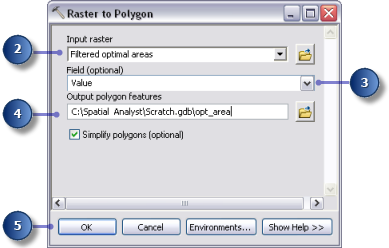
1. Open the Raster To Polygon tool in the Conversion Tools toolbox, in the From Raster toolset.
2. Click the Input raster drop-down arrow and click the Filtered optimal areas raster layer.
3. Leave the default for the Field parameter as VALUE.
4. Accept the default Output polygon features parameter path, but change the name to opt_area.
5. Leave the default checked to Simplify polygons. The polygons will be simplified to reduce the stair-step effect when a raster is converted to a polygon.
6. Click OK.

   

Executing the Select By Location tool

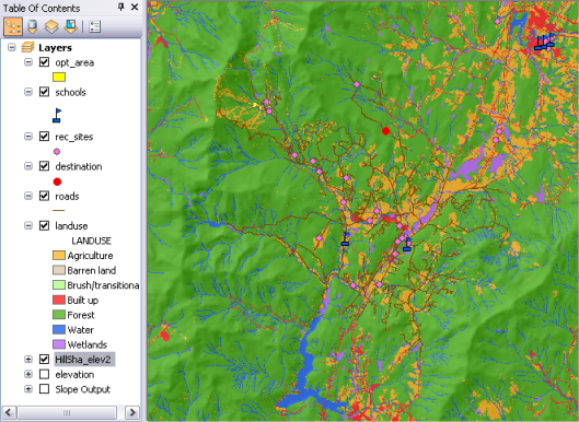
1. Leave the landuse, elevation, hillshade, destination, roads, rec_sites, schools, Slope Output, and opt_area layers in the table of contents. In the table of contents, right-click the layers to be removed, and click Remove. Press and hold the Shift key to select multiple layers. Your ArcMap table of contents display should resemble the following screen capture:

   

2. Open the Select Layer By Location tool in the Data Management toolbox, in the Layers and Table Views toolset.
3. For Input Feature Layer, choose opt_area from the drop-down list.
4. For the Relationship parameter, accept the default, which is INTERSECT.
5. Click the Selecting Features drop-down arrow and click the Roads layer.
6. Accept the default for the Selection type parameter, which is NEW_SELECTION.
7. Click OK.

   

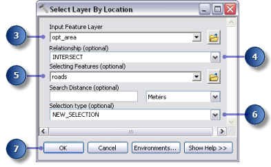
   All features that intersect roads are selected in the display.

Executing the Select Layer By Attribute tool

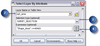
1. Open the Select Layer By Attribute tool in the Data Management toolbox, in the Layers and Table Views toolset.
2. For Layer Name of Table View, choose opt_area from the drop-down list.
3. For the Selection type parameter, choose SUBSET_SELECTION.
4. Click the query builder button.

   

5. Double-click Shape_Area in the list of fields to enter the field into the expression text box.
6. Click the greater than or equal to button .
7. Type 40469.
8. Click OK, then click OK again.

   

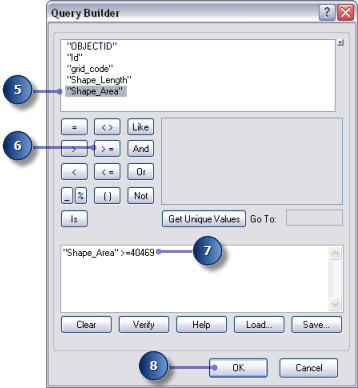
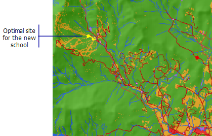
   There is one feature that fits the criteria of being equal to or greater than 10 acres (40,469 square meters).

Executing the Copy Features tool

1. Open the Copy Features tool in the Data Management toolbox, in the Features toolset.
2. Click the Input Features drop-down arrow and click the opt_area layer.
3. Click the browse button next to the Output Feature Class parameter and browse to C:\Spatial Analyst\Stowe.gdb. This stores your final result in your Stowe.gdb instead of your Scratch.gdb.
4. Type final_site for the name of the output feature class then click Save.
5. Click OK to run the tool.

   

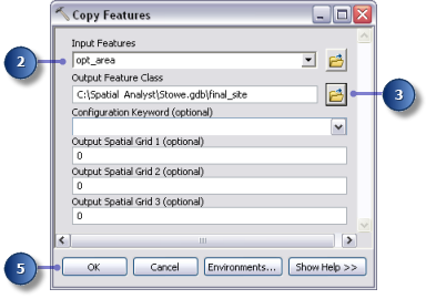
6. Right-click opt_area in the table of contents and click Remove.

   The final_site layer displays the location of the optimal site for the new school.

   

7. On the Standard toolbar, click the Save button .

Summary

You have now completed exercise 3. You can proceed to exercise 4, or you can stop and continue later.