Multi-Distance Spatial Cluster Analysis (Ripley's K Function)

Summary

Determines whether features, or the values associated with features, exhibit statistically significant clustering or dispersion over a range of distances.

Learn more about how Multi-Distance Spatial Cluster Analysis works

Illustration

Measure of spatial clustering/dispersion over a range of distances.

Usage

• This tool requires projected data to accurately measure distances.

• Tool output is a table with fields: ExpectedK and ObservedK containing the expected and observed K values, respectively. Because the L(d) transformation is applied, the ExpectedK values will always match the Distance value. A field named DiffK contains the Observed K values minus the Expected K values. If a confidence interval option is specified, two additional fields named LwConfEnv and HiConfEnv will be included in the Output Table as well. These fields contain confidence interval information for each iteration of the tool, as specified by the Number of Distance Bands parameter. The K function will optionally create a graph layer summarizing results.

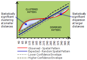
• When the observed K value is larger than the expected K value for a particular distance, the distribution is more clustered than a random distribution at that distance (scale of analysis). When the observed K value is smaller than the expected K value, the distribution is more dispersed than a random distribution at that distance. When the observed K value is larger than the HiConfEnv value, spatial clustering for that distance is statistically significant. When the observed K value is smaller than the LwConfEnv value, spatial dispersion for that distance is statistically significant. Additional information about interpretation is found in How Multi-Distance Spatial Cluster Analysis (Ripley's K-function) works .

• Enable the Display Results Graphically parameter to create a line graph summarizing tool results. The expected results will be represented by a blue line while the observed results will be a red line. Deviation of the observed line above the expected line indicates that the dataset is exhibiting clustering at that distance. Deviation of the observed line below the expected line indicates that the dataset is exhibiting dispersion at that distance. The line graph is created as a graph layer; graph layers are temporary and will be deleted when you close ArcMap. If you right-click the graph layer and select Save, the graph can be written to a Graph File. If you save your map document after saving your graph, a link to the graph file will be saved with your .mxd. For more information about graph files, see Exploring and visualizing data with graphs.

• For line and polygon features, feature centroids are used in distance computations. For multipoints, polylines, or polygons with multiple parts, the centroid is computed using the weighted mean center of all feature parts. The weighting for point features is 1, for line features is length, and for polygon features is area.

• The Weight Field is most appropriately used when it represents the number of incidents or counts.

• When no Weight Field is specified, the largest DiffK value tells you the distance where spatial processes promoting clustering are most pronounced.

• The following explains how the confidence envelope is computed:

  • No Weight Field

    When no Weight Field is specified, the confidence envelope is constructed by distributing points randomly in the study area and calculating L(d) for that distribution. Each random distribution of the points is called a "permutation". If 99_PERMUTATIONS is selected, for example, the tool will randomly distribute the set of points 99 times for each iteration. After distributing the points 99 times the tool selects, for each distance, the Observed k value that deviated above and below the Expected k value by the greatest amount; these values become the confidence interval.

  • Including a Weight Field

    When a Weight Field is specified, only the weight values are randomly redistributed to compute confidence envelopes; the point locations remain fixed. In essence, when a Weight Field is specified, locations remain fixed and the tool evaluates the clustering of feature values in space. On the other hand, when no Weight Field is specified the tool analyzes clustering/dispersion of feature locations.

• Because the confidence envelope is constructed from random permutations, the values defining the confidence envelope will change from one run to the next, even when parameters are identical. If you set a seed value, however, for the Random Number Generator geoprocessing environment, repeat analyses will produce consistent results.

• The number of permutations selected for the Compute Confidence Envelope parameter may be loosely translated to confidence levels: 9 for 90%, 99 for 99%, and 999 for 99.9%.

• When no study area is specified, the tool uses a minimum enclosing rectangle as the study area polygon. Unlike the extent, a minimum enclosing rectangle will not necessarily align with the x- and y-axes.

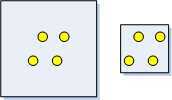
• The k-function statistic is very sensitive to the size of the study area. Identical arrangements of points can exhibit clustering or dispersion depending on the size of the study area enclosing them. Therefore, it is imperative that the study area boundaries are carefully considered. The picture below is a classic example of how identical feature distributions can be dispersed or clustered depending on the study area specified.

  

• A study area feature class is required if USER_PROVIDED_STUDY_AREA_FEATURE_CLASS is chosen for the Study Area Method parameter.

• If a Study Area Feature Class is specified, it should have exactly one single part feature (the study area polygon).

• If no Beginning Distance or Distance Increment is specified, then default values are calculated for you based on the extent of the Input Feature Class.

• The K function has an undercount bias for features located near the study area boundary. The Boundary Correction Method parameter provides methods for addressing this bias.

  • NONE

    No specific boundary correction is applied. However, points in the Input Feature Class that fall outside the user-specified study area are used in neighbor counts. This method is appropriate if you've collected data from a very large study area but only need to analyze smaller areas well within the boundaries of data collection.

  • SIMULATE_OUTER_BOUNDARY_VALUES

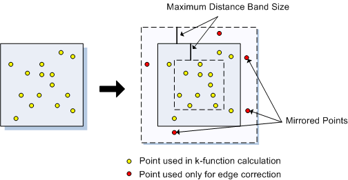
    This method creates points outside the study area boundary that mirror those found inside the boundary in order to correct for underestimates near the edges. Points that are within a distance equal to the maximum distance band of an edge of the study area are mirrored. The mirrored points are used so that edge points will have more accurate neighbor estimates. The diagram below illustrates what points will be used in the calculation and which will be used only for edge correction.

    

  • REDUCE_ANALYSIS_AREA

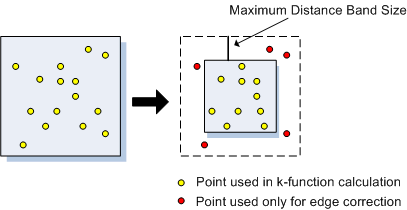
    This edge correction technique shrinks the size of the analysis area by a distance equal to the largest distance band to be used in the analysis. After shrinking the study area, points found outside of the new study area will be considered only when neighbor counts are being assessed for points still inside the study area. They will not be used in any other way during the k-function calculation. The diagram below illustrates which points will be used in the calculation and which will be used only for edge correction.

    

  • RIPLEY'S_EDGE_CORRECTION_FORMULA

    This method checks each point's distance from the edge of the study area and its distance to each of its neighbors. All neighbors that are further away from the point in question than the edge of the study area are given extra weighting. This edge correction method is only appropriate for square or rectangular shaped study areas, or when you select MINIMUM_ENCLOSING_RECTANGLE for the Study Area Method parameter.

• When no boundary correction is applied, the undercount bias increases as the analysis distance increases. If you enable the Display Results Graphically parameter, you will notice that the ObservedK line droops at the larger distances.

• Mathematically, the Multi-Distance Spatial Cluster Analysis tool uses a common transformation of Ripley's k-function where the expected result with a random set of points is equal to the input distance. The transformation L(d) is shown below.

  

  where A is area, N is the number of points, d is the distance and k(i, j) is the weight, which (if there is no boundary correction) is 1 when the distance between i and j is less than or equal to d and 0 when the distance between i and j is greater than d. When edge correction is applied, the weight of k(i, j) is modified slightly.

• Map layers can be used to define the Input Feature Class. When using a layer with a selection, only the selected features are included in the analysis.

Caution:

When using shapefiles, keep in mind that they cannot store null values. Tools or other procedures that create shapefiles from nonshapefile inputs may store or interpret null values as zero. In some cases, nulls are stored as very large negative values in shapefiles. This can lead to unexpected results. See Geoprocessing considerations for shapefile output for more information.

Syntax

MultiDistanceSpatialClustering_stats (Input_Feature_Class, Output_Table, Number_of_Distance_Bands, {Compute_Confidence_Envelope}, {Display_Results_Graphically}, {Weight_Field}, {Beginning_Distance}, {Distance_Increment}, {Boundary_Correction_Method}, {Study_Area_Method}, {Study_Area_Feature_Class})

Parameter	Explanation	Data Type
Input_Feature_Class	The feature class upon which the analysis will be performed.	Feature Layer
Output_Table	The table to which the results of the analysis will be written.	Table
Number_of_Distance_Bands	The number of times to increment the neighborhood size and analyze the dataset for clustering. The starting point and size of the increment are specified in the Beginning_Distance and Distance_Increment parameters, respectively.	Long
Compute_Confidence_Envelope (Optional)	The confidence envelope is calculated by randomly placing feature points (or feature values) in the study area. The number of points/values randomly placed is equal to the number of points in the feature class. Each set of random placements is called a permutation and the confidence envelope is created from these permutations. This parameter allows you to select how many permutations you want to use to create the confidence envelope. 0_PERMUTATIONS_-_NO_CONFIDENCE_ENVELOPE —Confidence envelopes are not created. 9_PERMUTATIONS —Nine sets of points/values are randomly placed. 99_PERMUTATIONS —99 sets of points/values are randomly placed. 999_PERMUTATIONS —999 sets of points/values are randomly placed.	String
Display_Results_Graphically (Optional)	Specifies whether the tool will create a graph layer summarizing results. NO_DISPLAY —No graphical summary will be created (default). DISPLAY_IT —A graphical summary will be created as a graph layer.	Boolean
Weight_Field (Optional)	A numeric field with weights representing the number of features/events at each location.	Field
Beginning_Distance (Optional)	The distance at which to start the cluster analysis and the distance from which to increment. The value entered for this parameter should be in the units of the Output Coordinate System.	Double
Distance_Increment (Optional)	The distance to increment during each iteration. The distance used in the analysis starts at the Beginning_Distance and increments by the amount specified in the Distance_Increment. The value entered for this parameter should be in the units of the Output Coordinate System environment setting.	Double
Boundary_Correction_Method (Optional)	Method to use to correct for underestimates in the number of neighbors for features near the edges of the study area. NONE —No edge correction is applied. However, if the input feature class already has points that fall outside the study area boundaries, these will be used in neighborhood counts for features near boundaries. SIMULATE_OUTER_BOUNDARY_VALUES —This method simulates points outside the study area so that the number of neighbors near edges is not underestimated. The simulated points are the "mirrors" of points near edges within the study area boundary. REDUCE_ANALYSIS_AREA —This method shrinks the study area such that some points are found outside of the study area boundary. Points found outside the study area are used to calculate neighbor counts but are not used in the cluster analysis itself. RIPLEY_EDGE_CORRECTION_FORMULA —For all the points (j) in the neighborhood of point i, this method checks to see if the edge of the study area is closer to i, or if j is closer to i. If j is closer, extra weight is given to the point j. This edge correction method is only appropriate for square or rectangular shaped study areas.	String
Study_Area_Method (Optional)	Specifies the region to use for the study area. The K Function is sensitive to changes in study area size so careful selection of this value is important. MINIMUM_ENCLOSING_RECTANGLE —Indicates that the smallest possible rectangle enclosing all of the points will be used. USER_PROVIDED_STUDY_AREA_FEATURE_CLASS —Indicates that a feature class defining the study area will be provided in the Study Area Feature Class parameter.	String
Study_Area_Feature_Class (Optional)	Feature class that delineates the area over which the input feature class should be analyzed. Only specified if Study_Area_Method = "USER_PROVIDED_STUDY_AREA_FEATURE_CLASS" .	Feature Layer

Derived Output

Name	Explanation	Data Type
Result_Image

Code sample

Multi-DistanceSpatialClusterAnalysis Example (Python Window)

The following Python Window script demonstrates how to use the Multi-DistanceSpatialClusterAnalysis tool.

import arcpy
arcpy.env.workspace = r"C:\data"
arcpy.MultiDistanceSpatialClustering_stats("911Calls.shp","kFunResult.dbf", 11,
                                           "0_PERMUTATIONS_-_NO_CONFIDENCE_ENVELOPE",
                                           "NO_DISPLAY", "#", 1000, 200,"REDUCE_ANALYSIS_AREA",
                                           "MINIMUM_ENCLOSING_RECTANGLE", "#")

Multi-DistanceSpatialClusterAnalysis Example (stand-alone Python script)

The following stand-alone Python script demonstrates how to use the Multi-DistanceSpatialClusterAnalysis tool.

# Use Ripley's K-Function to analyze the spatial distribution of 911
# calls in Portland Oregon 

# Import system modules
import arcpy

# Set property to overwrite existing outputs
arcpy.env.overwriteOutput = True

# Local variables...
workspace = r"C:\Data"

try:
    # Set the current workspace (to avoid having to specify the full path to the feature classes each time)
    arcpy.env.workspace = workspace

    # Set Distance Band Parameters: Analyze clustering of 911 calls from
    # 1000 to 3000 feet by 200 foot increments
    numDistances = 11
    startDistance = 1000.0
    increment = 200.0

    # Process: Run K-Function...
    kFun = arcpy.MultiDistanceSpatialClustering_stats("911Calls.shp",
                        "kFunResult.dbf", numDistances,
                        "0_PERMUTATIONS_-_NO_CONFIDENCE_ENVELOPE", 
                        "NO_DISPLAY", "#", startDistance, increment,
                        "REDUCE_ANALYSIS_AREA",
                        "MINIMUM_ENCLOSING_RECTANGLE", "#")

except:
    # If an error occurred when running the tool, print out the error message.
    print(arcpy.GetMessages())

Environments

• Output Coordinate System

  Note:

  Feature geometry is projected to the Output Coordinate System prior to analysis, so values entered for the Beginning Distance and Distance Increment parameters should match those specified in the Output Coordinate System. All mathematical computations are based on the Output Coordinate System spatial reference.

• Geographic Transformations
• Current Workspace
• Scratch Workspace
• Random number generator

Licensing information

• ArcGIS Desktop Basic: Yes
• ArcGIS Desktop Standard: Yes
• ArcGIS Desktop Advanced: Yes