ArcGIS supports display of raster and TIN surface models and provides analysis tools in the Spatial Analyst, 3D Analyst, and Geostatistical Analyst extensions to create, analyze, and extract information from surfaces.
What are surfaces?
Surfaces represent phenomena that have values at every point across their extent. The values at the infinite number of points across the surface are derived from a limited set of sample values. These may be based on direct measurement, such as height values for an elevation surface, or temperature values for a temperature surface; between these measured locations, values are assigned to the surface by interpolation. Surfaces can also be mathematically derived from other data, such as slope and aspect surfaces derived from an elevation surface, a surface of distance from bus stops in a city, or surfaces showing concentration of criminal activity or probability of lightning strikes.
- Surfaces can be represented using contour lines or isolines, arrays of points, TINs, and rasters; however, most surface analysis in GIS is done on raster or TIN data.
- Contours are sets of lines of equal value across a surface. They are frequently created to represent surfaces on a map.
- Points can be regularly or irregularly distributed across a surface. They are usually used as input to interpolation, kriging, or triangulation tools to create raster or TIN surfaces, though they are also sometimes used for cartographic representation of a surface such as wind direction flags or least-cost direction arrows.
- TINs are nets of triangular facets defined by nodes and edges that cover a surface. TINs are constructed from a set of known values, or spot heights, that are used as initial nodes in the triangulation. Lines where the shape of the surface abruptly changes, such as ridgelines, streams, or roads, can be incorporated into TINs as breaklines, and areas that share a value can be incorporated as fill polygons. The values at locations between nodes can be derived for a TIN using linear interpolation from the nearest nodes. TINs are usually used to represent terrain surfaces in engineering applications, as the spot heights can be irregularly distributed to accommodate areas of high variability in the surface, and their values and exact positions are retained as nodes in the TIN.
- Rasters are rectangular arrays of cells (or pixels), each of which stores a value for the part of the surface it covers. A given cell contains a single value, so the amount of detail that can be represented for the surface is limited to the size of the raster cells. Rasters are the most commonly used surface models in ArcGIS. The simplicity of the raster data structure makes calculations on rasters (or comparisons between rasters) faster for rasters than other surface representations. Rasters are also used to store imagery; scanned maps; and categorical information, such as land-use class, which is often derived from imagery.
Creating surfaces
In ArcGIS, there are tools to create surfaces from vector features or from other surfaces. There are several ways to create surfaces, including interpolating values stored at measured point locations, interpolating a surface of the density of a given phenomenon or feature type from the numbers of features in an area, deriving surfaces of distance (or direction) from a feature or features, or deriving a surface from another surface (slope raster from elevation).
Interpolation tools
Interpolation tools create a continuous surface from discrete samples with measured values, such as elevation or chemical concentration. There are several interpolation tools, and each has a variety of parameters that influence the resulting surface.
Below is an example of how different interpolation techniques can produce different output surfaces from the same input data.
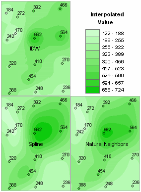
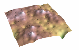
The simplest interpolation tools are Inverse Distance Weighted (IDW) and Natural Neighbor interpolation. These estimate surface values for each cell using the value and distance of nearby points. The interpolated values for IDW surfaces are a weighted average of the values of a set of nearby points, weighted so the influence of nearby points is greater than that of distant points (that is, with the inverse of the distance).
Below is an example of a surface interpolated from point values using IDW interpolation.
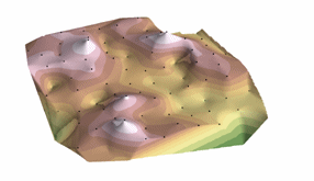
Natural Neighbors interpolation is like IDW interpolation, except that the data points used to interpolate the surface values for each cell are identified and weighted using a Delauney triangulation, as in a TIN. Natural Neighbors interpolation reliably works with much larger datasets than the other interpolation methods.
Below is an example of a surface interpolated from point values using Natural Neighbors interpolation.
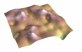
Spline and Trend interpolation interpolate best-fit surfaces to the sample points using polynomial and least-squares methods, respectively. Spline interpolation fits a mathematical surface through the points that minimizes sharp bending; it is useful for surfaces that vary smoothly, such as water table heights.
Below is an example of a surface interpolated from point values using Spline interpolation.
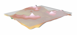
Trend surfaces are good for identifying coarse scale patterns in data; the interpolated surface rarely passes through the sample points.
Below is an example of a Trend surface for a set of points, in transparent gray, and the IDW interpolated surface for the same points.
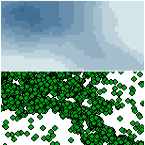
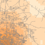
Density tools produce a surface that represents how much or how many of some thing there are per unit area. You might use density surfaces to represent the distribution of a wildlife population from a set of observations, or the degree of urbanization of an area based on the density of roads. There are density tools for point and line features.
Below are examples of density surfaces interpolated from point and line features.
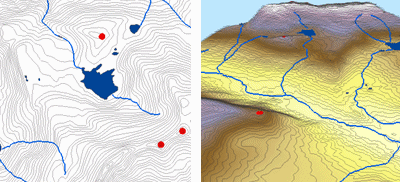
Topo To Raster is a specialized tool for creating hydrologically correct raster surfaces from vector data of terrain components such as elevation points, contour lines, stream lines, lake polygons, sink points, and study area boundary polygons.
Below is an example of a surface interpolated from elevation points, contour lines, stream lines, and lake polygons using Topo To Raster interpolation.
TIN surface creation tools include Create TIN and Edit TIN, which are used to initially create a TIN for a specific area and to add vector features to it, and Raster To TIN, which converts a raster surface model to a TIN surface model.
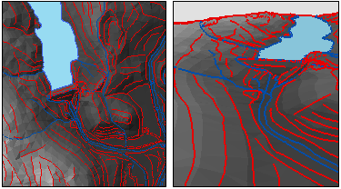
Below is an example of a TIN surface created from point, line, and polygon features. The terrain heights are derived from spot sample elevations at the vertices of many of the triangular facets. The shape of the TIN surface is controlled by the triangulation of these spot heights with breaklines (the blue stream and red ridgelines and slope breaks) and with the blue reservoir fill polygon.
Geostatistical interpolation techniques are derived from statistics. They allow the creation of predicted value surfaces and the interpretation of levels of certainty about the predictions. Kriging is an advanced surface creation technique that is most useful when there is a spatially correlated distance or directional bias in the data. It is most used in soil science and geology. Geostatistical geoprocessing tools and a wizard for Geostatistics are available with the Geostatistical Analyst extension.
The Geostatistical Analyst wizard allows surface creation by Kriging, as well as Cokriging, Radial Basis Function, Inverse Distance Weighted, Global Polynomial, and Local Polynomial interpolation methods. It also includes tools for data exploration, such as histograms, normal QQ plots, and trend analysis. The Geostatistical Analyst also includes tools for data preparation such as the creation of subsets of large datasets, data transformation, and data detrending.
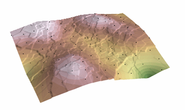
Below is an example of a surface interpolated from point values using Kriging.
Analyzing surfaces
Surface analysis involves several kinds of processing, including extracting new surfaces from existing surfaces, reclassifying surfaces, and combining surfaces.
Certain tools extract or derive information from a surface, a combination of surfaces, or surfaces and vector data.
Terrain analysis tools
Some of these tools are primarily designed for the analysis of raster terrain surfaces. These include Slope, Aspect, Hillshade, and Curvature tools.
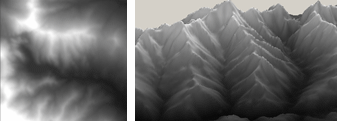
Below is an example of an elevation raster in planimetric and perspective views.

The Slope tool calculates the maximum rate of change from a cell to its neighbors, which is typically used to indicate the steepness of terrain.
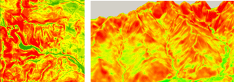
Below is an example of an Slope raster in planimetric and perspective views.

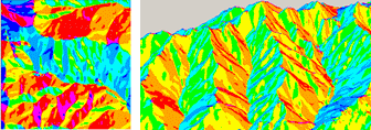
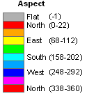
The Aspect tool calculates the direction in which the plane fitted to the slope faces for each cell. The aspect of a surface typically affects the amount of sunlight it receives (as does the slope); in northern latitudes places with a southerly aspect tend to be warmer and drier than places that have a northerly aspect.
Below is an example of an aspect raster in planimetric and perspective views.
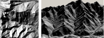
Hillshade shows the intensity of lighting on a surface given a light source at a particular location; it can model which parts of a surface would be shadowed by other parts.
Below is an example of a hillshade raster in planimetric and perspective views.

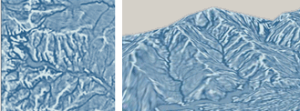
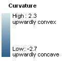
Curvature calculates the slope of the slope (the second derivative of the surface), that is, whether a given part of a surface is convex or concave. Convex parts of surfaces, like ridges, are generally exposed and drain to other areas. Concave parts of surfaces, like channels, are generally more sheltered and accept drainage from other areas. The Curvature tool has a couple of optional variants, Plan and Profile Curvature. These are used primarily to interpret the effect of terrain on water flow and erosion. The profile curvature affects the acceleration and deceleration of flow, which influence erosion and deposition. The planiform curvature influences convergence and divergence of flow.
Below is an example of a curvature raster in planimetric and perspective views.
Visibility tools
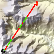
Some tools are used to analyze the visibility of parts of surfaces. The Line Of Sight tool identifies whether or not one location is visible from another, and whether or not the intervening locations along a line between the two locations are visible.
Below is an example of a Line of Sight analysis. An observer at the southern end of the line can see the parts of the terrain along the line that are colored green, and cannot see the parts of the terrain along the line that are colored red. In this case, the observer cannot see the fire in the valley on the other side of the mountain.

The visibility tools support offsets, which allow you to specify the height of the observer points and the observed points or cells.
Below is an example of a Line Of Sight analysis comparing the results with no offset and with a target offset. Locations along the line that are visible to the observer are green, and those that are hidden by intervening terrain are red.
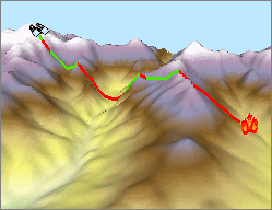

You might use a target offset to model a building or a smoke plume.
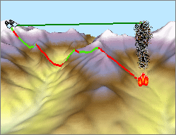

With a large target offset, the target is visible, even though the visibility of the points along the intervening terrain do not change.
You could add an offset to the observer as well, to model a tower at the observer location. Adding an observer offset generally increases the amount of terrain that is visible from a location.
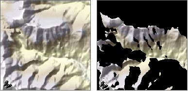
The Observer Points tool identifies which observers, specified as a set of points, can see any given cell of a raster surface. The Viewshed tool calculates, for each cell of a raster surface and a set of input points (or the vertices of input lines), how many observers can see any given cell.
Below is an example of a Viewshed analysis with a single input observer point. The observer has an offset to model the view from a fire tower 50 meters taller than the ground surface. Cells outside the observer's viewshed are blacked out in the image on the right.

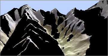
In the perspective views below, you can see the observer point and the terrain.
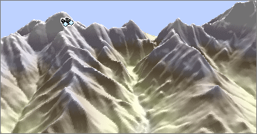
Ridges hide the valleys behind them from the observer point.

Both the Observer Points and Viewshed tools also allow you to specify observer and target offsets, as well as a set of parameters that let you limit the directions and distance that each observer can view.
Volume tools
Some tools are used to calculate volumes from surface information. These tools calculate the difference in volume between a raster or TIN surface and another surface. Depending on the tool, the other surface might be specified by a horizontal plane at a given elevation or by a second raster or TIN surface.
Below is an example of a terrain surface representing the typical fill level of a reservoir. You could use the volume tools to calculate the volume of additional water when the reservoir is near capacity.
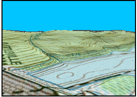
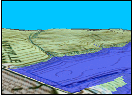
The Surface Volume tool is used to calculate volume of a surface above or below a horizontal plane at a specific elevation. You might use this tool to calculate the volume of water in a section of river channel at a particular flood stage. This tool can be used on raster or TIN surfaces. The output of the tool is a text file reporting the parameters used and the resulting surface area and volumes.
The Cut Fill tool is used to calculate the amount of difference in each cell for a before and after raster of the same area. This tool could be used to calculate the volume of earth that must be brought to or removed from a construction site to reshape a surface. This tool works on two rasters, and the results are presented as a raster of the difference between the two layers.
The TIN Difference tool is similar to the Cut/Fill tool, but it works on a pair of input TIN surfaces. This tool creates a polygon feature class where each polygon is given attributes identifying whether the second TIN is above, below, or the same as the first TIN and the volume of the difference between the TINs in that polygon.
The TIN Polygon Volume tool calculates the volume difference and surface area for each polygon in a feature class relative to a TIN surface. Each polygon in the feature class represents a horizontal area at an elevation specified in a height field. The volume above or below this planar area to the TIN surface is added to a volume field in the feature class, and the surface area of the polygon is added to a surface area field.
Reclassification tools
One way to convert surface data into more usable information for an analysis is to reclassify the surface. Reclassifying a surface sets a range of values equal to a single value. You might reclassify a surface so that areas with cells above a given value, or between two critical values, are given one code, and other areas are given another; or, you might use the Reclassify (or Slice) tool to divide a surface up into a given number of classes as a means of aggregating and generalizing detailed data. Reclassifying surfaces is often done to reduce the number of output categories for an overlay analysis.
Below is an example of an elevation raster sliced into several classes (each class represents a range of elevation values) and reclassified into two classes (above and below a given elevation).

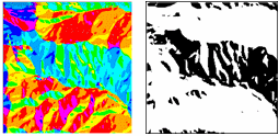
Below is an example of an aspect raster reclassified into two classes; south and southwest aspect slopes have a value of 1 (light), and other aspects have a value of 0 (dark).
Distance tools
Some distance tools create rasters that show the distance of each cell from a set of locations.
The tools include the shortest straight-line distance to a set of source features and the direction of the closest feature. The Euclidean Allocation tool creates zones of a surface that are allocated to the closest feature.
The Cost Distance, Cost Path, Cost Back Link, and Cost Allocation tools are used to find the shortest (least cost) path from sources to destinations, taking into account a raster that quantifies the cost of traversing the surface. The cost raster may reflect difficulty, energy, time, or dollar costs or a unitless composite of several factors that influence the cost of travel or flow across a surface. The Path set of tools perform much the same function as the Cost set but take the additional factors of surface distance and vertical travel difficulty (cost) into account; that is, the fact that the length of a given line over hilly terrain is longer than the same line on a perfectly flat surface and the fact that it may be easier to move along a slope than it is to move up or down the slope.
For more information about the Distance tools, see the Proximity Analysis section.
Overlay tools
Raster overlay tools combine two or more rasters using logical, arithmetic, or weighted combination methods. The Weighted Overlay and Weighted Sum tools allows you to combine multiple rasters of varying importance. This is useful in site suitability analyses when several factors contribute to suitability, but certain factors contribute more heavily than others.
Some tools perform algebraic or logical operations upon surfaces. The Spatial Analyst Neighborhood tools, such as the block and focal functions, compute values for the cells of an output raster based on the values of surrounding cells; these can be used to remove noise or enhance edge contrasts, or resample rasters to a lower resolution. Local functions combine, compare, or summarize several rasters on a cell by cell basis. Zonal functions calculate for each cell some function or statistic using the value for all cells belonging to the same zone.
Extracting information from surfaces
Some tools extract vector features from surfaces, or produce tabular summaries or smaller raster samples of surfaces.
Sampling rasters
The Sample tool creates a table that shows the values of a raster, or several rasters, at a set of sample point locations. The points can be in a point feature class or the cells in a raster that have values other than NoData. You might use this tool to get information about what occurs at a set of points, such as bird nesting sites, from terrain, distance to water, and forest type rasters.
Below is an example of a geology raster being sampled at a set of points; the result is a table.
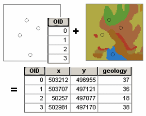
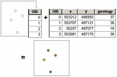
The output table can be analyzed on its own or joined to the sample point features.
Below is an example of the sample results table joined back to the original sample points.
The Extract tools create a new raster with a copy of the cells within some mask area. The Extract By Mask tool lets you use a polygon feature class to extract the raster data.
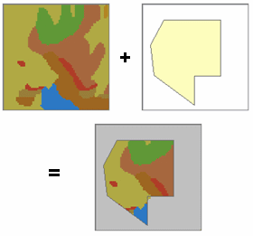
The Extract Values To Points tool creates a new feature class of points with the values of a single raster at a set of input point features. The Extract By Attributes tool selects cells of a raster based on a logical query. Extract By Polygon and Extract By Rectangle take lists of coordinate values that define an area and output a raster that is either inside or outside the polygon. Extract By Circle takes the center coordinates and radius of a circle and outputs a raster that is either inside or outside the circle. Extract By Points takes a list of coordinate values that define a set of points and outputs a raster of the cell values at these points (or excluding these points). In all cases, the cells from the original raster that are not part of the Extract area are given NoData values. The 3D Analyst Surface Spot tool extracts elevation values from a surface for a set of point features and adds them to a Spot attribute of the points.
Extracting information from a TIN
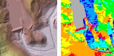
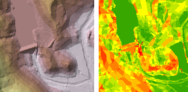
TINs store slope and aspect information as attributes of the TIN facets. Rather than deriving slope and aspect for TIN surfaces (as you do with raster terrain models, which only store the elevation values), you simply need to extract that information from the facets to a set of polygons. TIN Aspect and TIN Slope extract aspect and slope data from a TIN and add that information as attributes of a polygon feature class.
Below is an example of TIN elevation model and the aspect information it contains:

Below is an example of TIN elevation model and the slope information it contains:

Extracting contours
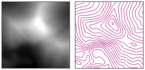
The Contour tool extracts lines of constant value (isolines) from a raster surface. The TIN Contour tool extracts a line feature class of contours from a TIN surface.
Below is an example of an elevation model and contour lines extracted from it.
Zonal statistics tools can produce tables of summary statistics for a given raster based on zones defined by another raster or a polygon feature class, or it can produce a new raster that corresponds to the zones with a specific summary statistic as an attribute.
Hydrology tools
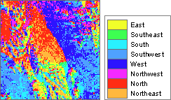
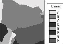
Hydrology tools derive drainage basin and stream information from terrain rasters; this information can be converted to vector features. The process requires several tools that derive information from the terrain surface, resulting in basin and stream rasters that can be converted to vector features. The Flow Direction tool takes a terrain surface and identifies the down-slope direction for each cell. The Basin tool uses the results of the Flow Direction tool to identify the drainage basins, made up of the connected cells that drain to a common location. The Flow Accumulation tool identifies how much surface flow accumulates in each cell; cells with high accumulation values are usually stream or river channels. It also identifies local topographic highs (areas of zero flow accumulation) such as mountain peaks and ridgelines.
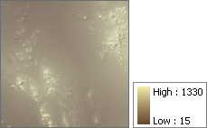
Below is an example of an elevation model:
Below is an example of a flow direction surface derived from the elevation model:
Below is an example of basins derived from the flow direction surface:
Below is an example of a flow accumulation surface derived from the flow direction surface:
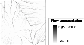
The flow accumulation surface can be processed with a Map Algebra Conditional (Con) statement such as:
con (flowacc > 100, 1)
to capture only those cells with high flow accumulation values (in this case, greater than 100) into a stream raster.
Below is an example of a stream raster extracted from the flow accumulation surface:
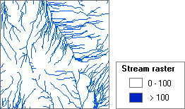
The Stream To Feature tool creates vector stream line features from a stream raster and a flow direction surface.