Available with 3D Analyst license.
Forest canopy density and height are used as variables in a number of environmental applications, such as biomass estimation, vegetation coverage, and biodiversity determination. Canopy density, or canopy cover, is the ratio of vegetation to ground as seen from the air. Canopy height measures how far above the ground the top of the canopy is. Lidar can be used to determine both of these variables.
The following are steps to calculate canopy density and height from lidar points. First, you need lidar that has been classified into ground returns (bare earth) versus non-ground returns. This type of point classification is usually performed by your data provider. Secondly, you need to consider when the lidar was collected and the type of vegetation in the study area. If there are a lot of deciduous trees and the collection was performed during autumn (leaf off), the density calculation is not going to work.
Create a LAS dataset and layer
The LAS dataset can be used to calculate canopy density and height. Use the Create LAS Dataset geoprocessing tool to reference your LAS format lidar data. See the Alternate Workflow section at the end of this topic if you're working with ASCII data or you want to work with your LAS-based points in a geodatabase. Once the LAS dataset is made, use a layer to define filter properties that will control which points in the LAS files get used. To make a layer add the dataset to a map or run the Make LAS Dataset Layer geoprocessing tool. When defining the layer, select all the returns, then focus on the class codes. Basically, we'll be working with two sets of points: those on the ground and those above ground. LAS points are typically classified by the schema defined in the LAS 1.1 standard outlined by the American Society for Photogrammetry and Remote Sensing (ASPRS):
ASPRS Standard Lidar Point Classes
| Classification Code | Classification type |
|---|---|
0 | Never classified |
1 | Unassigned |
2 | Ground |
3 | Low Vegetation |
4 | Medium Vegetation |
5 | High Vegetation |
6 | Building |
7 | Noise |
8 | Model Key |
9 | Water |
10 | Reserved for ASPRS Definition |
11 | Reserved for ASPRS Definition |
12 | Overlap |
13–31 | Reserved for ASPRS Definition |
Calculating the density
The most effective way to determine the canopy density is to divide the study area into many small equal-sized units through rasterization. In each raster cell, you compare the number of above ground points to the total number of points.
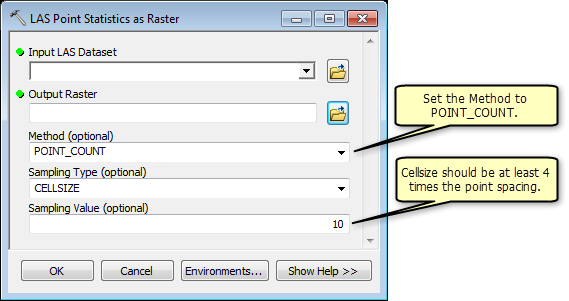
The important technique to remember here is to determine an appropriate cellsize for this analysis. It needs to be at least four times the average point spacing. You can go larger but not smaller with the cell size.
- Use the LAS Point Statistics As Raster geoprocessing tool on the above ground points with the POINT_ COUNT option.
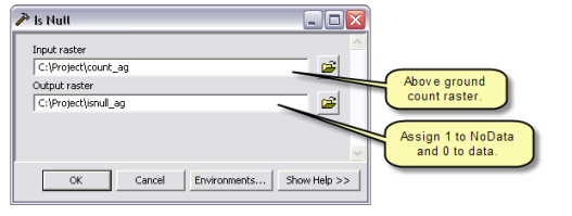
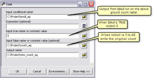
- Convert any resulting NoData cells to 0 so that subsequent operations treat a cell with no points as 0. This is accomplished using the IsNull geoprocessing tool followed by the Con geoprocessing tool.
- Repeat steps 1 and 2 with the lidar ground multipoints.
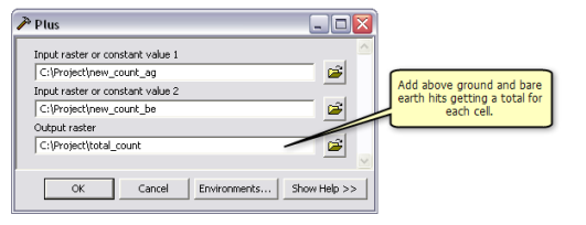
- Add the aboveground and bare earth rasters together to get a total count per cell using the Plus geoprocessing tool.
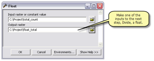
- All the rasters you've made so far are long data types. You need one raster to be floating point to get floating-point output from the Divide geoprocessing tool that you will use in step 6. To generate a float raster, use the output raster from the Plus geoprocessing tool as input to the Float geoprocessing tool.
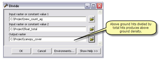
- Now use the Divide geoprocessing tool to compare the aboveground count raster and the floating-point total count raster. This gives you the ratio from 0.0 to 1.0, where 0.0 represents no canopy and 1.0 very dense canopy.
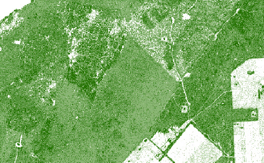
The following image represents canopy density. The lightest areas have little to no vegetation. These are areas where a large percentage of lidar shots could see the ground. The dark green areas, where lidar could not penetrate to ground as well, indicate denser vegetation canopy.
Calculating the height
To determine canopy height, you will need to subtract the bare earth surface (DEM) from the first return surface (DSM). Follow the steps in the Creating raster DEMs and DSMs from large lidar point collections topic to generate these two surfaces.
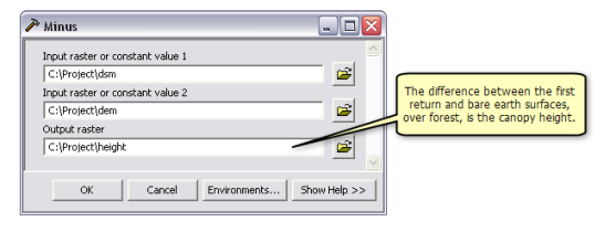
- Once you have generated the first return and bare earth rasters, use the Minus geoprocessing tool to determine the difference between these two raster datasets. The difference results represent, over forest, the canopy height.
The image below represents height above ground. It ranges from blue (little to no height) to orange, which is the tallest.
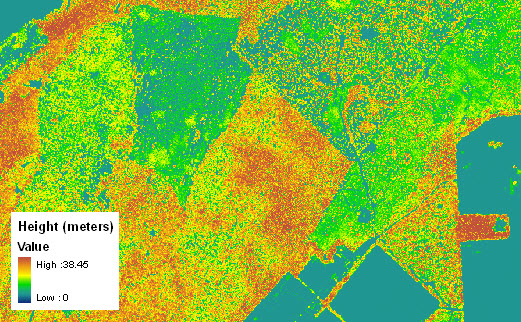
Lidar can be used to calculate the density and height of vegetation. This is useful for a variety of purposes, including biomass and carbon estimates, as well as forest management.
Alternative Workflow
If your lidar points are in ASCII format you need to have two sets of files: those containing only the ground points and those containing only the non-ground points. If your files are organized like this, then you should load the points into multipoint feature classes in a geodatabase using the ASCII 3D To Feature Class geoprocessing tool. Run it twice, once for each set of files. Then run the Point To Raster geoprocessing tool as a substitute for the LAS Point Statistics tool used in the LAS dataset based workflow outlined above.
If you have LAS format data but prefer to load just the points of interest into a geodatabase and work from them, use the LAS To Multipoint geoprocessing tool two times. Do it once to load the ground points then again to load the non-ground points. Then run the Point To Raster geoprocessing tool as a substitute for the LAS Point Statistics tool used in the LAS dataset-based workflow outlined above.