Disponible avec une licence Geostatistical Analyst.
Kriging methods depend on mathematical and statistical models. The addition of a statistical model that includes probability separates kriging methods from the deterministic methods described in Deterministic methods for spatial interpolation. For kriging, you associate some probability with your predictions; that is, the values are not perfectly predictable from a statistical model. Consider the example of a sample of measured nitrogen values in a field. Obviously, even with a large sample, you will not be able to predict the exact value of nitrogen at some unmeasured location. Therefore, you not only try to predict it, but you also assess the error of the prediction.
Kriging methods rely on the notion of autocorrelation. Correlation is usually thought of as the tendency for two types of variables to be related. For example, the stock market tends to make positive changes with lower interest rates, so it's said that they are negatively correlated. However, the stock market is positively autocorrelated, which means it has correlation within itself. In the stock market, two values will tend to be more similar if they are only one day apart as opposed to being one year apart. This is related to a basic principle of geography—things closer together tend to be more similar than those that are farther apart. The rate at which the correlation decays can be expressed as a function of distance.
Autocorrelation is a function of distance. This is a defining feature of geostatistics. In classical statistics, observations are assumed independent, that is, there is no correlation between observations. In geostatistics, the information on spatial locations allows you to compute distances between observations and to model autocorrelation as a function of distance.
Also notice that, in general, the stock market goes up with time, and this is termed trend. For geostatistical data, you have the same terms, and they are expressed in the following simple mathematical formula:
Z(s) = µ(s) + ε(s),where Z(s) is the variable of interest, decomposed into a deterministic trend µ(s) and a random, autocorrelated errors form ε(s). The symbol s simply indicates the location; think of it as containing the spatial x- (longitude) and y- (latitude) coordinates. Variations on this formula form the basis for all the different types of kriging. Start on the right and move left.
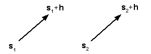
No matter how complicated the trend in the model is, µ(s) still will not predict perfectly. In this case, some assumptions about the error term ε(s) are made; namely, you would expect them to be 0 (on average) and that the autocorrelation between ε(s) and ε(s + h) does not depend on the actual location s but only the displacement h between the two. This is necessary to ensure replication so you can estimate the autocorrelation function. For example, in the following figure:

random errors at location pairs connected by the arrows are assumed to have the same autocorrelation.
Next, examine the trend. It can be a simple constant, that is, µ(s) = m for all locations s, and if µ is unknown, this is the model on which ordinary kriging is based. It can also be composed of a linear function of the spatial coordinates themselves, for example:
µ(s) = ß0 + ß1x + ß2y + ß3x2 + ß4y2 + ß5xy,where this is a second-order polynomial trend surface and is just linear regression on the spatial x- and y-coordinates. Trends that vary, and where the regression coefficients are unknown, form models for universal kriging. Whenever the trend is completely known (that is, all parameters and covariates known), whether constant or not, it forms the model for simple kriging.
Now, look at the left side of the decomposition, Z(s) = µ(s) + ε(s). You can perform transformations on Z(s). For example, you can change it to an indicator variable, where it is 0 if Z(s) is below some value (for example, 0.12 ppm for ozone concentration) or 1 if it is above some value. You may want to predict the probability that Z(s) is above the threshold value, and predictions based on this model form indicator kriging. You can make general unspecified transformations of the Z(s) and call them fi(Z(si)) for the ith variable. You can form predictors of functions of variables; for example, if you want to predict at location s0, you form the disjunctive kriging predictor of g(Z(s0)) using data fi(Z(si)).
Finally, consider the case where you have more than one variable type, and you form the models Zj(s) = µj(s) + εj(s) for the jth variable type. Here, you can consider a different trend for each variable, and besides autocorrelation for the errors εj(s), you also have cross-correlation between the errors εj(s) and εk(s) for the two variable types. For example, you can consider the cross-correlation between two variables like ozone concentration and particulate matter, and they need not be measured at the same locations. Models based on more than one variable of interest form the basis of cokriging. You can form an indicator variable of Z(s), and if you predict it using the original untransformed data Z(s) in a cokriging model, you obtain probability kriging. If you have more than one variable of interest, you can consider ordinary cokriging, universal cokriging, simple cokriging, indicator cokriging, probability cokriging, and disjunctive cokriging as multivariate extensions of the different types of kriging described earlier.
Vous avez un commentaire à formuler concernant cette rubrique ?