Summary
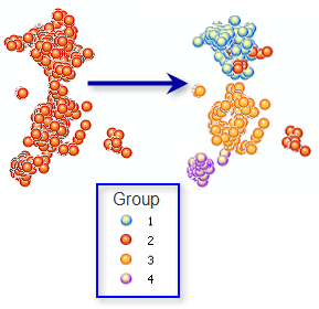
Groups features based on feature attributes and optional spatial/temporal constraints.
Illustration

Usage
-
This tool produces an output feature class with the fields used in the analysis plus a new integer field named SS_GROUP. Default rendering is based on the SS_GROUP field and shows you which group each feature falls into. If you indicate that you want 3 groups, for example, each record will contain a 1, 2, or 3 for the SS_GROUP field. When NO_SPATIAL_CONSTRAINT is selected for the Spatial Constraints parameter, the output feature class will also contain a new binary field called SS_SEED. The SS_SEED field indicates which features were used as starting points to grow groups. The number of nonzero values in the SS_SEED field will match the value you entered for the Number of Groups parameter.
-
This tool will optionally create a PDF report file when you specify a path for the Output Report File parameter. This report contains a variety of tables and graphs to help you understand the characteristics of the groups identified. The PDF report file is accessible through the Results window.
-
When the Input Feature Class is not projected (that is, when coordinates are given in degrees, minutes, and seconds) or when the output coordinate system is set to a Geographic Coordinate System, distances are computed using chordal measurements. Chordal distance measurements are used because they can be computed quickly and provide very good estimates of true geodesic distances, at least for points within about thirty degrees of each other. Chordal distances are based on an oblate spheroid. Given any two points on the earth's surface, the chordal distance between them is the length of a line, passing through the three-dimensional earth, to connect those two points. Chordal distances are reported in meters.
-
The Unique ID Field provides a way for you to link records in the Output Feature Class back to data in the original input feature class. Consequently, the Unique ID Field values must be unique for every feature, and typically should be a permanent field that remains with the feature class. If you don't have a Unique ID Field in your dataset, you can easily create one by adding a new integer field to your feature class table and calculating the field values to be equal to the FID/OID field. You cannot use the FID/OID field directly for the Unique ID Field parameter.
-
The Analysis Fields should be numeric and should contain a variety of values. Fields with no variation (that is, the same value for every record) will be dropped from the analysis but will be included in the Output Feature Class. Categorical fields may be used with the Grouping Analysis tool if they are represented as dummy variables (a value of one for all features in a category and zeros for all other features).
-
The Grouping Analysis tool will construct groups with or without space or time constraints. For some applications you may not want to impose contiguity or other proximity requirements on the groups created. In those cases you will set the Spatial Constraints parameter to NO_SPATIAL_CONSTRAINT.
-
For some analyses, you will want groups to be spatially contiguous. The contiguity options are enabled for polygon feature classes and indicate features can only be part of the same group if they share an edge (CONTIGUITY_EDGES_ONLY) or if they share either an edge or a vertex (CONTIGUITY_EDGES_CORNERS) with another member of the group.
-
The DELAUNAY_TRIANGULATION and K_NEAREST_NEIGHBORS options are appropriate for point or polygon features when you want to ensure all group members are proximal. These options indicate that a feature will only be included in a group if at least one other feature is a natural neighbor (Delaunay Triangulation) or a K Nearest Neighbor. K is the number of neighbors to consider and is specified using the Number of Neighbors parameter.
-
In order to create groups with both space and time constraints, use the Generate Spatial Weights Matrix tool to first create a spatial weights matrix file (.swm) defining the space-time relationships among your features. Next run Grouping Analysis setting the Spatial Constraints parameter to GET_SPATIAL_WEIGHTS_FROM_FILE and the Spatial Weights Matrix File parameter to the SWM file you created.
-
Additional Spatial Constraints, such as fixed distance, may be imposed by using the Generate Spatial Weights Matrix tool to first create an SWM file and then providing the path to that file for the Spatial Weights Matrix File parameter.
-
Defining a spatial constraint ensures compact, contiguous, or proximal groups. Including spatial variables in your list of Analysis Fields can also encourage these group attributes. Examples of spatial variables would be distance to freeway on-ramps, accessibility to job openings, proximity to shopping opportunities, measures of connectivity, and even coordinates (X, Y). Including variables representing time, day of the week, or temporal distance can encourage temporal compactness among group members.
-
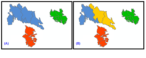
When there is a distinct spatial pattern to your features (an example would be three separate, spatially distinct clusters), it can complicate the spatially constrained grouping algorithm. Consequently, the grouping algorithm first determines if there are any disconnected groups. If the number of disconnected groups is larger than the Number of Groups specified, the tool cannot solve and will fail with an appropriate error message. If the number of disconnected groups is exactly the same as the Number of Groups specified, the spatial configuration of the features alone determines group results, as shown in (A) below. If the Number of Groups specified is larger than the number of disconnected groups, grouping begins with the disconnected groups already determined. For example, if there are three disconnected groups and the Number of Groups specified is 4, one of the three groups will be divided to create a fourth group, as shown in (B) below.

-
In some cases, the Grouping Analysis tool will not be able to meet the spatial constraints imposed, and some features will not be included with any group (the SS_GROUP value will be -9999 with hollow rendering). This happens if there are features with no neighbors. To avoid this, use K_NEAREST_NEIGHBORS which ensures all features have neighbors. Increasing the Number of Neighbors parameter will help resolve issues with disconnected groups.
-
While there is a tendency to want to include as many Analysis Fields as possible, for this tool it works best to start with a single variable and build. Results are much easier to interpret with fewer analysis fields. It is also easier to determine which variables are the best discriminators when there are fewer fields.
-
When you select NO_SPATIAL_CONSTRAINT for the Spatial Constraints parameter, you have three options for the Initialization Method: FIND_SEED_LOCATIONS, GET_SEEDS_FROM_FIELD, and USE_RANDOM_SEEDS. Seeds are the features used to grow individual groups. If, for example, you enter a 3 for the Number of Groups parameter, the analysis will begin with three seed features. The default option, FIND_SEED_LOCATIONS, randomly selects the first seed and makes sure that the subsequent seeds selected represent features that are far away from each other in data space. Selecting initial seeds that capture different areas of data space improves performance. Sometimes, you know that specific features reflect distinct characteristics that you want represented by different groups. In that case, create a seed field to identify those distinctive features. The seed field you create should have zeros for all but the initial seed features; the initial seed features should have a value of 1. You will then select GET_SEEDS_FROM_FIELD for the Initialization Method parameter. If you are interested in doing some kind of sensitivity analysis to see which features are always found in the same group, you might select the USE_RANDOM_SEEDS option for the Initialization Method parameter. For this option, all of the seed features are randomly selected.
-
Any values of 1 in the Initialization Field will be interpreted as a seed. If there are more seed features than Number of Groups, the seed features will be randomly selected from those identified by the Initialization Field. If there are fewer seed features than specified by Number of Groups, the additional seed features will be selected so they are far away (in data space) from those identified by the Initialization Field.
-
Sometimes you know the Number of Groups most appropriate for your data. In the case that you don't, however, you may have to try different numbers of groups, noting which values provide the best group differentiation. When you check the Evaluate Optimal Number of Groups parameter, a pseudo F-statistic will be computed for grouping solutions with 2 through 15 groups. If no other criteria guide your choice for Number of Groups, use a number associated with one of the largest pseudo F-statistic values. The largest F-statistic values indicate solutions that perform best at maximizing both within-group similarities and between-group differences. When you specify an optional Output Report File, that PDF report will include a graph showing the F-statistic values for solutions with 2 through 15 groups.
-
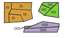
Regardless of the Number of Groups you specify, the tool will stop if division into additional groups becomes arbitrary. Suppose, for example, that your data consists of three spatially clustered polygons and a single analysis field. If all the features in a cluster have the same analysis field value, it becomes arbitrary how any one of the individual clusters is divided after three groups have been created. If you specify more than three groups in this situation, the tool will still only create three groups. As long as at least one of the analysis fields in a group has some variation of values, division into additional groups can continue.

Groups will not be divided further if there is no variation in the analysis field values -
When you include a spatial or space-time constraint in your analysis, the pseudo F-Statistics are comparable (as long as the Input Features and Analysis Fields don't change). Consequently, you can use the F-Statistic values to determine not only optimal Number of Groups, but also to help you make choices about the most effective Spatial Constraints option, Distance Method, and Number of Neighbors.
-
The K-Means algorithm used to partition features into groups when NO_SPATIAL_CONSTRAINT is selected for the Spatial Constraints parameter and FIND_SEED_LOCATIONS or USE_RANDOM_SEEDS is selected for the Initialization Method incorporates heuristics and may return a different result each time you run the tool (even using the same data and the same tool parameters). This is because there is a random component to finding the initial seed features used to grow the groups.
-
When a spatial constraint is imposed, there is no random component to the algorithm, so a single pseudo F-Statistic can be computed for groups 2 through 15, and the highest F-Statistic values can be used to determine the optimal Number of Groups for your analysis. Because the NO_SPATIAL_CONSTRAINT option is a heuristic solution, however, determining the optimal number of groups is more involved. The F-Statistic may be different each time the tool is run, due to different initial seed features. When a distinct pattern exists in your data, however, solutions from one run to the next will be more consistent. Consequently, to help determine the optimal number of groups when the NO_SPATIAL_CONSTRAINT option is selected, the tool solves the grouping analysis 10 times for 2, 3, 4, and up to 15 groups. Information about the distribution of these 10 solutions is then reported (min, max, mean, and median) to help you determine an optimal number of groups for your analysis.
-
The Grouping Analysis tool returns three derived output values for potential use in custom models and scripts. These are the pseudo F-Statistic for the Number of Groups (Output_FStat), the largest pseudo F-Statistic for groups 2 through 15 (Max_FStat), and the number of groups associated with the largest pseudo F-Statistic value (Max_FStat_Group). When you do not elect to Evaluate Optimal Number of Groups, all of the derived output variables are set to None.
-
The group number assigned to a set of features may change from one run to the next. For example, suppose you partition features into two groups based on an income variable. The first time you run the analysis you might see the high income features labeled as group 2 and the low income features labeled as group 1; the second time you run the same analysis, the high income features might be labeled as group 1. You might also see that some of the middle income features switch group membership from one run to another when NO_SPATIAL_CONSTRAINT is specified.
-
While you can select to create a very large number of different groups, in most scenarios you will likely be partitioning features into just a few groups. Because the graphs and maps become difficult to interpret with lots of groups, no report is created when you enter a value larger than 15 for the Number of Groups parameter or select more than 15 Analysis Fields. You can increase this limitation on the maximum number of groups, however.
-
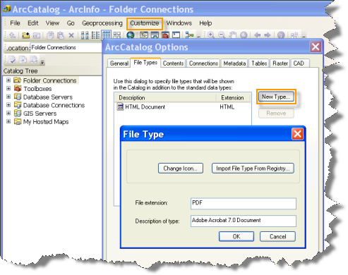
This tool will optionally create a PDF report summarizing results. PDF files do not automatically appear in the Catalog window. If you want PDF files to be displayed in Catalog, open the ArcCatalog application, select the Customize menu option, click ArcCatalog Options, and select the File Types tab. Click on the New Type button and specify PDF, as shown below, for File Extension.

-
On machines configured with the ArcGIS language packages for Chinese or Japanese, you might notice missing text or formatting problems in the PDF Output Report File. These problems can be corrected by changing the font settings.
-
For more information about the Output Report File, see Learn more about how Grouping Analysis works.
Syntax
GroupingAnalysis_stats (Input_Features, Unique_ID_Field, Output_Feature_Class, Number_of_Groups, Analysis_Fields, Spatial_Constraints, {Distance_Method}, {Number_of_Neighbors}, {Weights_Matrix_File}, {Initialization_Method}, {Initialization_Field}, {Output_Report_File}, {Evaluate_Optimal_Number_of_Groups})| Parameter | Explanation | Data Type |
Input_Features | The feature class or feature layer for which you want to create groups. | Feature Layer |
Unique_ID_Field | An integer field containing a different value for every feature in the input feature class. If you don't have a Unique ID field, you can create one by adding an integer field to your feature class table and calculating the field values to equal the FID or OBJECTID field. | Field |
Output_Feature_Class | The new output feature class created containing all features, the analysis fields specified, and a field indicating which group each feature belongs to. | Feature Class |
Number_of_Groups | The number of groups to create. The Output Report parameter will be disabled for more than 15 groups. | Long |
Analysis_Fields [analysis_field,...] | A list of fields you want to use to distinguish one group from another. The Output Report parameter will be disabled for more than 15 fields. | Field |
Spatial_Constraints | Specifies if and how spatial relationships among features should constrain the groups created.
| String |
Distance_Method (Optional) | Specifies how distances are calculated from each feature to neighboring features.
| String |
Number_of_Neighbors (Optional) | This parameter may be specified whenever the Spatial_Constraints parameter is K_NEAREST_NEIGHBORS or one of the contiguity methods (CONTIGUITY_EDGES_ONLY or CONTIGUITY_EDGES_CORNERS). The default number of neighbors is 8 and cannot be smaller than 2 for K_NEAREST_NEIGHBORS. This value reflects the exact number of nearest neighbor candidates to consider when building groups. A feature will not be included in a group unless one of the other features in that group is a K nearest neighbor. The default for CONTIGUITY_EDGES_ONLY and CONTIGUITY_EDGES_CORNERS is 0. For the contiguity methods, this value reflects the minimum number of neighbor candidates to consider. Additional nearby neighbors for features with less than the Number_of_Neighbors specified will be based on feature centroid proximity. | Long |
Weights_Matrix_File (Optional) | The path to a file containing spatial weights that define spatial relationships among features. | File |
Initialization_Method (Optional) | Specifies how initial seeds are obtained when the Spatial_Constraint parameter selected is NO_SPATIAL_CONSTRAINT. Seeds are used to grow groups. If you indicate you want three groups, for example, the analysis will begin with three seeds.
| String |
Initialization_Field (Optional) | The numeric field identifying seed features. Features with a value of 1 for this field will be used to grow groups. | Field |
Output_Report_File (Optional) | The full path for the PDF report file to be created summarizing group characteristics. This report provides a number of graphs to help you compare the characteristics of each group. Creating the report file can add substantial processing time. | File |
Evaluate_Optimal_Number_of_Groups (Optional) |
| Boolean |
Code sample
GroupingAnalysis example 1 (Python window)
The following Python window script demonstrates how to use the GroupingAnalysis tool.
import arcpy
import arcpy.stats as SS
arcpy.env.workspace = r"C:\GA"
SS.GroupingAnalysis("Dist_Vandalism.shp", "TARGET_FID", "outGSF.shp", "4",
                    "Join_Count;TOTPOP_CY;VACANT_CY;UNEMP_CY",
                    "NO_SPATIAL_CONSRAINT", "EUCLIDEAN", "", "", "FIND_SEED_LOCATIONS", "",
                    "outGSF.pdf", "DO_NOT_EVALUATE")
GroupingAnalysis example 2 (stand-alone Python script)
The following stand-alone Python script demonstrates how to use the GroupingAnalysis tool.
# Grouping Analysis of Vandalism data in a metropolitan area
# using the Grouping Analysis Tool

# Import system modules
import arcpy, os
import arcpy.stats as SS

# Set geoprocessor object property to overwrite existing output, by default
arcpy.gp.overwriteOutput = True

try:
    # Set the current workspace (to avoid having to specify the full path to
    # the feature classes each time)
    arcpy.env.workspace = r"C:\GA"

    # Join the 911 Call Point feature class to the Block Group Polygon feature class
    # Process: Spatial Join
    fieldMappings = arcpy.FieldMappings()
    fieldMappings.addTable("ReportingDistricts.shp")
    fieldMappings.addTable("Vandalism2006.shp")

    sj = arcpy.SpatialJoin_analysis("ReportingDistricts.shp", "Vandalism2006.shp", "Dist_Vand.shp",
                               "JOIN_ONE_TO_ONE",
                               "KEEP_ALL",
                               fieldMappings,
                               "COMPLETELY_CONTAINS", "", "")

    # Use Grouping Analysis tool to create groups based on different variables or analysis fields
    # Process: Group Similar Features
    ga = SS.GroupingAnalysis("Dist_Vand.shp", "TARGET_FID", "outGSF.shp", "4",
                                       "Join_Count;TOTPOP_CY;VACANT_CY;UNEMP_CY",
                                       "NO_SPATIAL_CONSRAINT", "EUCLIDEAN", "", "", "FIND_SEED_LOCATIONS", "",
                                       "outGSF.pdf", "DO_NOT_EVALUATE")

    # Use Summary Statistic tool to get the Mean of variables used to group
    # Process: Summary Statistics
    SumStat = arcpy.Statistics_analysis("outGSF.shp", "outSS", "Join_Count MEAN; \
                               VACANT_CY MEAN;TOTPOP_CY MEAN;UNEMP_CY MEAN",
                                       "GSF_GROUP")

except:
    # If an error occurred when running the tool, print out the error message.
    print(arcpy.GetMessages())
Environments
Licensing information
- ArcGIS Desktop Basic: Yes
- ArcGIS Desktop Standard: Yes
- ArcGIS Desktop Advanced: Yes